7. Network Model Object
The network model defines the states of and connections between network elements, as well as the parameters and functions defining the relationships between states and port injections. This network model with a unified structure is the key to a flexible modular design where model elements can simply define a few parameters and all of the mathematics involved in computing injections and their derivatives for a given state is handled automatically.
One of the unique features of the network model is that the network model object, which contains network model elements, is a network model element itself. Each network model element can optionally define the following:
nodes to serve as network connection points
ports for connecting to network nodes
states which fully capture the element’s operating condition
There are two types of states that make up the element’s full state variable \(\X\), voltage states \(\V\) associated with each port, and optional non-voltage states \(\Z\). The network model object inherits from mp_idx_manager from MP-Opt-Model to track and index the nodes, ports, and states added by its elements, and the corresponding voltage and non-voltage state variables.
A given network model implements a specific network model formulation. Figure 7.1 shows the structure of an AC network model for an element with \(n_p\) connection ports and \(n_z\) non-voltage states.

Figure 7.1 AC Model for Element with \(n_p\) Ports
The MP-Element technical note, MATPOWER Technical Note 5 [TN5], includes a lot more detail on the network model and especially on the mathematics involved in the model formulations.
7.1. Network Model Formulations
Each concrete network model element class, including the container class, inherits from a specific subclass of mp.form. That is, it implements a specific network model formulation. For example, Figure 7.2 shows the corresponding classes for the three network model formulations currently implemented, (1) DC, (2) AC with cartesian voltage representation, and (3) AC with polar voltage representation.

Figure 7.2 Network Model Formulation Classes
By convention, network model formulation class names begin with mp.form. It is the formulation class that defines the network model’s parameters and methods for accessing them. It also defines the form of the state variables, real or complex, and methods for computing injections as a function of the state, and in the case of nonlinear formulations, corresponding derivatives as well.
All formulations share a common structure, illustrated in Figure 7.1, with ports, corresponding voltage states, non-voltage states, and functions of predefined form for computing port injections from the state.
7.1.1. DC Formulation
For the DC formulation, the state vector \(\x\) is real valued and the port injection function is defined in terms of active power injections. The state begins with the \(n_p \times 1\) vector \(\Va\) of voltage angles at the \(n_p\) ports, and may include an \(n_\z \times 1\) real vector of additional state variables \(\z\), for a total of \(n_\x\) state variables.
The port injection function in this case defines the active power port injections as a linear function of a set of parameters \(\BB\), \(\KK\) and \(\pv\), where \(\BB\) is an \(n_p \times n_p\) susceptance matrix, \(\KK\) is an \(n_p \times n_\z\) matrix coefficient for a linear power injection function, and \(\pv\) is an \(n_p \times 1\) constant power injection.
7.1.2. AC Formulations
For the AC formulations, the state vector \(\X\) is complex valued and there are two port injection functions, one for complex power injections and one for current injections, as shown in Figure 7.1. The state begins with the \(n_p \times 1\) vector \(\V\) of complex voltages at the \(n_p\) ports, and may include an \(n_\Z \times 1\) real vector of additional state variables \(\Z\), for a total of \(n_\X\) state variables.
The port injection functions for the model, both complex power injection \(\GS(\X)\) and complex current injection \(\GI(\X)\), are defined by three terms, a linear current injection component \(\Ilin(\X)\), a linear power injection component \(\Slin(\X)\), and an arbitrary nonlinear component, \(\Snln(\X)\) or \(\Inln(\X)\), respectively.
The linear current and power injection components are expressed in terms of the six parameters, \(\YY\), \(\LL\), \(\MM\), \(\NN\), \(\iv\), and \(\sv\). The admittance matrix \(\YY\) and linear power coefficient matrix \(\MM\) are \(n_p \times n_p\), linear coefficient matrices \(\LL\) and \(\NN\) are \(n_p \times n_\Z\), and \(\iv\) and \(\sv\) are \(n_p \times 1\) vectors of constant current and power injections, respectively.
Note that the arbitrary nonlinear injection component, represented by either \(\Snln(\X)\) or \(\Inln(\X)\), corresponds to a single set of injections represented either as a complex power injection or as a complex current injection, but not both. Since the functions represent the same set of injections, they are not additive components, but rather must be related to one another by the following relationship.
Complex Power Injections
Then the port injection function for complex power can be written as follows.
Complex Current Injections
Similarly, the port injection function for complex current can be written as follows.
The derivatives of \(\Snln\) and \(\Inln\) are assumed to be provided explicitly, and the derivatives of the other terms of (7.7) and (7.8) are derived in [TN5].
7.2. Network Models
A network model object is primarily a container for network model element objects and is itself a network model element. All network model classes inherit from mp.net_model and therefore also from mp.element_container, mp_idx_manager, and mp.nm_element. Concrete network model classes are also formulation-specific, inheriting from a corresponding subclass of mp.form as shown in Figure 7.3.
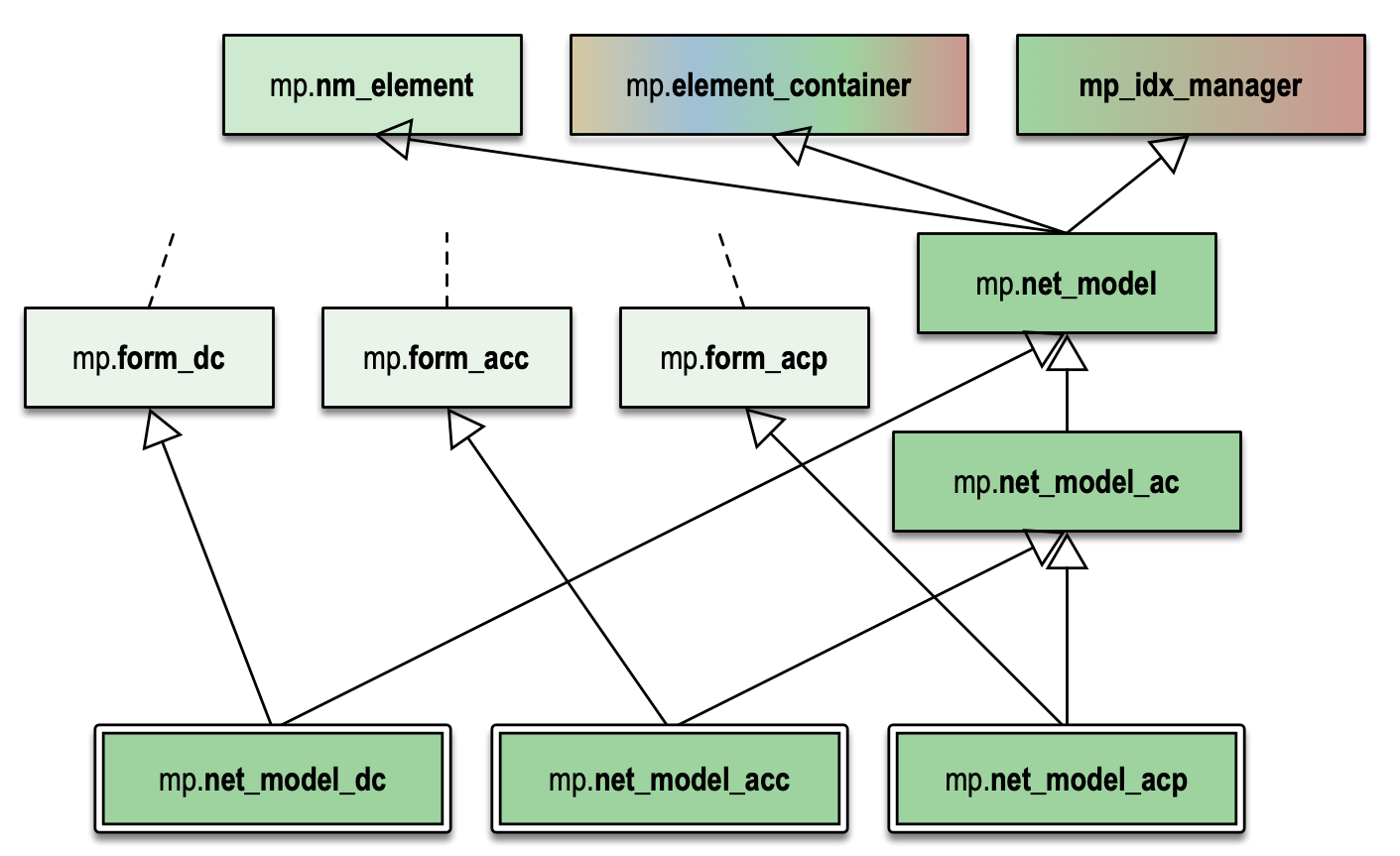
Figure 7.3 Network Model Classes
By convention, network model variables are named nm and network model class names begin with mp.net_model.
7.2.1. Building a Network Model
A network model object is created in two steps. The first is to call the constructor of the desired network model class, without arguments. This initializes the element_classes property with a list of network model element classes. This list can be modified before the second step, which is to call the build() method, passing in the data model object.
nm = mp.net_model_acp();
nm.build(dm);
The build() method proceeds through the following stages sequentially, looping through each element at each stage.
Create – Instantiate each element object.
Count and add - For each element object, determine the number of online elements from the corresponding data model element and, if nonzero, store it in the object and add the object to the
elementsproperty of thenm.Add nodes – Allow each element to add network nodes, then add voltage variables for each node.
Add states – Allow each element to add non-voltage states, then add non-voltage variables for each state.
Build parameters – Construct the formulation-specific model parameters for each element, including mappings of element port to network node and element non-voltage state to system non-voltage variable. Add ports to the container object for each element to track per-element port indexing.
7.2.2. Node Types
Most problems require that certain nodes be given special treatment depending on their type. For example, in the power flow problem, there is typically a single reference node, some PV nodes, with the rest being PQ nodes.
In the current design, each node-creating network model element class implements a node_types() method that returns information about the types of the nodes it creates. The container object node_types() method assembles that information for the full set of network nodes. It can also optionally, assign a new reference node if one does not exist. There are also methods, namely set_node_type_ref(), set_node_type_pv(), set_node_type_pq(), for setting the type of a network node and having the relevant elements update their corresponding data model elements.
7.3. Network Model Elements
A network model element object encapsulates all of the network model parameters for a particular element type. All network model element classes inherit from mp.nm_element and also, like the container, from a formulation-specific subclass of mp.form. Each element type typically implements its own subclasses, which are further subclassed per formulation. A given network model element object contains the aggregate network model parameters for all online instances of that element type, stored in the set of matrices and vectors that correspond to the formulation, e.g. \(\BB\), \(\KK\) and \(\pv\) from (7.2) for DC and \(\YY\), \(\LL\), \(\MM\), \(\NN\), \(\iv\), and \(\sv\) from (7.4) and (7.5) for AC.
So, for example, in a system with 1000 in-service transmission lines, the \(\YY\) parameter in the corresponding AC network model element object would be a 2000 \(\times\) 2000 matrix for an aggregate 2000-port element, representing the 1000 two-port transmission lines.
By convention, network model element variables are named nme and network model element class names begin with mp.nme. Figure 7.4 shows the inheritance relationships between a few example network model element classes. Here the mp.nme_bus_acp and mp.nme_gen_acp classes are used for all problems with an AC polar formulation, while the AC cartesian and DC formulations use their own respective subclasses.
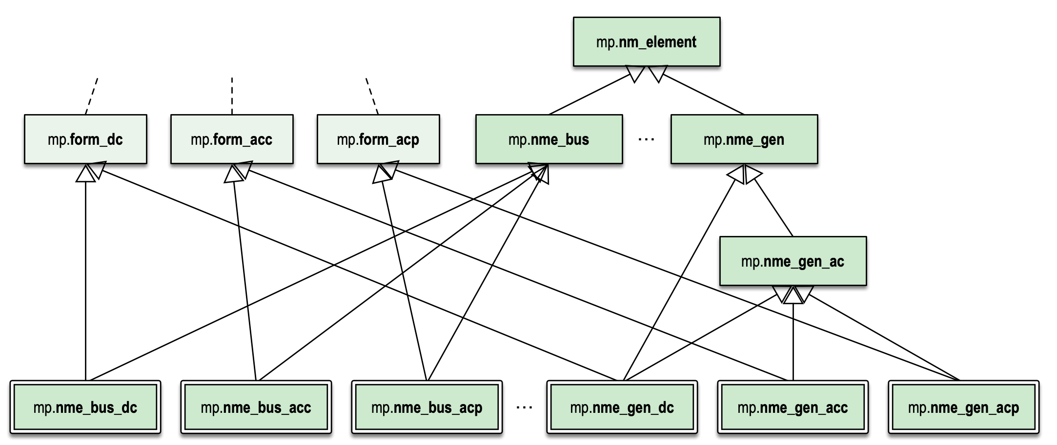
Figure 7.4 Network Model Element Classes
7.3.1. Example Elements
Here are brief descriptions of the network models for a few simple element types. There are other elements, and the point is that new elements are relatively simple to implement, simply by specifying the nodes, ports and states they add, and the parameters that define the relationships between the states and the port injections.
Bus
A bus element inherits from mp.nme_bus and defines a single node per in-service bus, with no ports or non-voltage states. So it has no model parameters.
Generator
A gen element is a 1-port element that inherits from mp.nme_gen and defines a single non-voltage state per in-service generator to represent the power injection. It connects to the node corresponding to a particular bus. The only non-zero parameters are \(\KK\) (DC) or \(\NN\) (AC), which are negative identity matrices, since the power injections (into the element) are the negative of the generated power.
Branch
A branch element is a 2-port element that inherits from mp.nme_branch with no nodes or non-voltage states. It connects to nodes corresponding to two particular buses. The only non-zero parameters are \(\BB\) and \(\pv\) (DC), or \(\YY\) (AC).
Load
A load element is a 1-port element that inherits from mp.nme_load with no ports or states. It connects to the node corresponding to a particular bus. For a simple constant power load, the only non-zero parameters are \(\pv\) (DC) or \(\sv\) (AC), equal to the power consumed by the load.
7.3.2. Building Element Parameters
Typically, a network model element builds parameters only for its in-service elements, stacking the corresponding parameters into vectors and matrices, with one row per element of that type. For the DC formulation, these are the three parameters \(\BB\), \(\KK\) and \(\pv\) from Section 7.1.1. For the AC formulations they are the six parameters, \(\YY\), \(\LL\), \(\MM\), \(\NN\), \(\iv\), and \(\sv\) from Section 7.1.2.
Take, for example, an AC model with two-port transmission lines modeled by a simple series admittance, where the two ports are labeled with \(f\) and \(t\). For line \(i\) with series admittance \(\cscal{y}^i_s\), we have
The individual admittance parameters for the \(n_k\) individual lines are then stacked as follows,
to form the admittance matrix parameter \(\YY\) that we see in (7.4) for the corresponding element object.
Stacking the individual port current and voltage variables,
results in the port injection currents from (7.8) for this aggregate element taking the form
When building its parameters, each network model element object also defines an element-node incidence matrix \(C\) for each of its ports and an element-variable incidence matrix \(D\) for each non-voltage states. For example, a transmission line element would define two \(C\) matrices, one mapping branches to their corresponding from bus and the other to their corresponding to bus.
7.3.3. Aggregation
Since the model parameters are consistent across all network model elements for a given formulation, and the connectivity of the elements is captured in the \(C\) and \(D\) incidence matrices for each element type, the network model object can assemble the parameters from all elements into a single aggregate network model characterized by parameters of the same form. This aggregate model can then be used to compute port or node injections from the aggregate system state, as well as any needed derivatives of these injection functions.
For more details on how the aggregation is done, see [TN5].