3. Architecture Overview
A new object-oriented MATPOWER core architecture (MP-Core), designed around the concept of a generic system element, [1] was introduced in MATPOWER 8.0, along with two frameworks for employing this new MP-Core in MATPOWER. This chapter gives an overview of this architecture.
MATPOWER’s primary function is to solve steady-state electric power system simulation and optimization problems, such as power flow, continuation power flow and optimal power flow. At the top level of MP-Core is a task object that constructs the various layers of modeling for the desired problem type and formulation, solves the problem, and propogates the solution back through the modeling layers to the user.
This architecture employs an explicit three-layer modeling structure designed to decouple from one another (1) the user-visible element parameters and quantities, (2) the network connections, states and flows, and (3) the mathematical problem being solved. The three layers are referred to, resepectively, as the data, network, and mathematical (or math) modeling layers as shown in Figure 3.1.
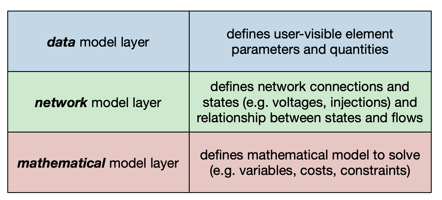
Figure 3.1 MATPOWER Model Layers
The data model layer is further decoupled from any particular data format, such as the legacy MATPOWER case struct (mpc) and case file formats, by introducing a data conversion service (data model converter) to convert data between the data model and specific external data formats.
Each modeling layer, plus the data conversion service, is organized around a collection of element objects, one for each element type, enclosed in a container object. An element type corresponds to a particular type of device (e.g. bus, generator, transmission line) or some other attribute or service (e.g. transmission interface, reserve requirement) in the system. This structure provides extraordinary flexibility by allowing the user to customize the environment by adding new, or modifying existing, element types independently from the rest.
3.1. MATPOWER Object Instances
In any given MATPOWER run, a set of object instances are created and used to solve the problem. The structure of these object instances in the object-oriented MATPOWER core architecture (MP-Core) is show in Figure 3.2. The classes for the various objects may be specific to (1) the type of problem being solved, (2) the problem formulation, (3) the data source, and for individual elements, (4) the type of element. The labels in the white circles in the figure are used by convention throughout the codebase in variable and class names for the corresponding type of object.
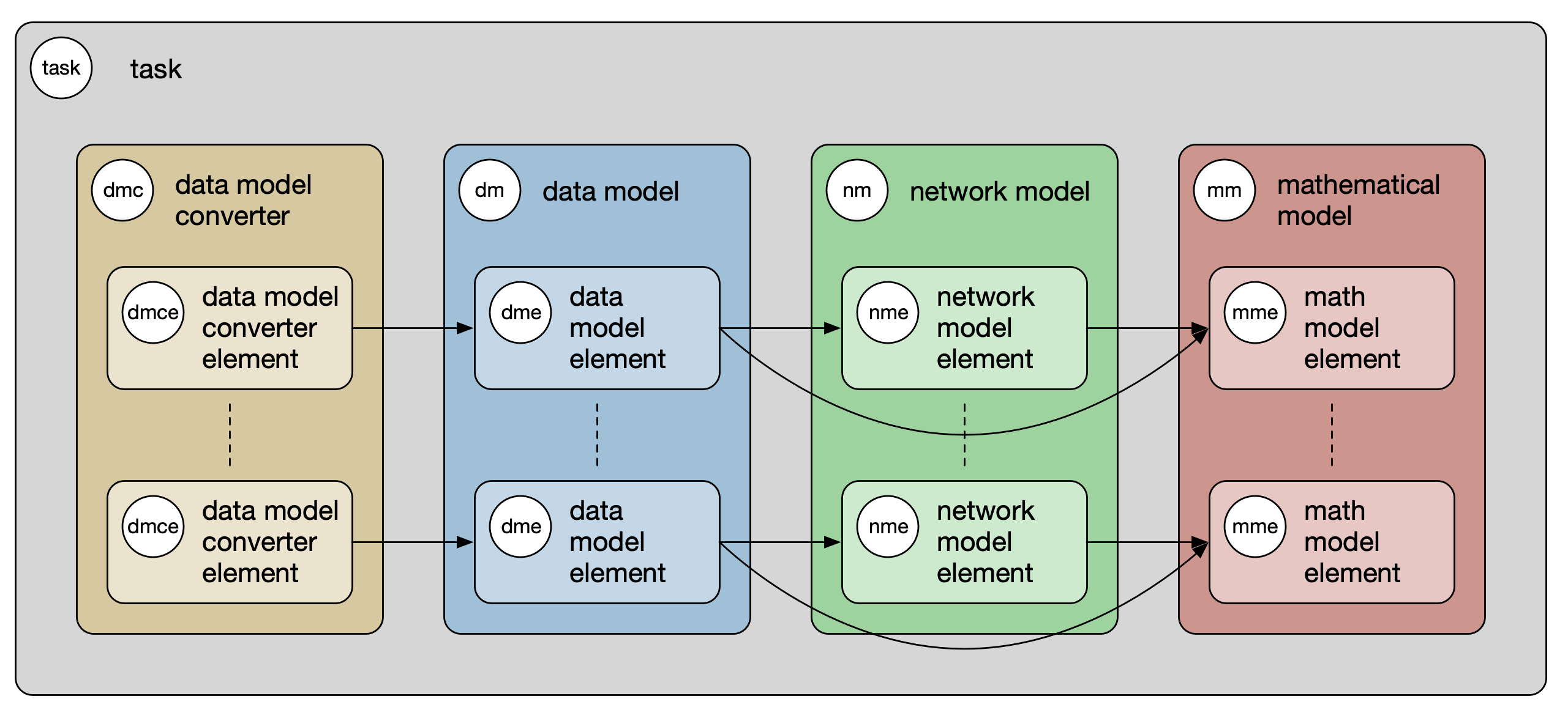
Figure 3.2 MATPOWER Object Instances
A single task object is created to manage the overall process. The task is specific to the type of problem being solved, e.g. power flow (PF), continuation power flow (CPF), or optimal power flow (OPF), and it has a run() method that sets up and solves the correspnding problem. For example, the following runs an OPF for the 9-bus case.
mpopt = mpoption('verbose', 2);     % set MATPOWER options
task = mp.task_opf();               % create task object for OPF
task.run('case9', mpopt);           % create and run task for 'case9'
The steps shown in Listing 3.1 are roughly equivalent to those performed when the task is run. It defines the classes used to construct each of the model objects, as well as the data model converter. In this example, the classes are defined explicitly, but in the actual code they are returned by calls to corresponding methods, allowing them to be overridden by subclasses.
The task then creates the data model converter object that corresponds to the data source provided, followed by the three main model objects. The data model is created from the specified data source with the help of the data model converter, and is then used to create the network model. The math model is then created using both the data and network models. After solving itself, the math model is also used to update the states of the other two model objects.
 1% define classes used to construct model objects and data model converter
 2dmc_class = @mp.dm_converter_mpc2;  % data model convert class, MATPOWER case format v2
 3dm_class = @mp.data_model_opf;      % data model class for OPF
 4nm_class = @mp.net_model_acp;       % network model class for AC polar
 5mm_class = @mp.math_model_opf_acps; % math model class for AC polar power OPF
 6
 7% create objects
 8dmc = dmc_class().build();              % create data model converter
 9dm = dm_class().build('case9', dmc);    % create data model for 'case9'
10nm = nm_class().build(dm);              % create network model
11mm = mm_class().build(nm, dm, mpopt);   % create math model
12
13% find solution
14opt = mm.solve_opts(nm, dm, mpopt);     % get solver options
15mm.solve(opt);                          % solve math model
16nm = mm.network_model_x_soln(nm);       % update network model state with soln
17nm.port_inj_soln();                     % use network model to compute flows
18dm = mm.data_model_update(nm, dm, mpopt);   % update data model with soln
Each of the four main objects created by the task consists of a container object holding a set of corresponding element objects. That is, the data model contains a set of data model elements, the network model, a set of network model elements, etc., one for each element type. Each element type is associated with a name, that is a valid struct field name used to identify the corresponding element in each container object. The list of element classes for a given container is defined by the container class, but can be modified after the container’s construction and before calling its build() method.
The build process of a given container object simply loops through its set of elements, building each one, possibly with access to the respective element of the other model layers. For example, when building the network model (nm), a network model element (nme) is constructed for each type of element, pulling its data from the corresponding data model element (dme). For example, the network model element for generators pulls its data from the data model element for generators.
3.2. MATPOWER Class Hierarchies
A summary of the class inheritance structure in MP-Core is represented in Figure 3.3, showing class name conventions, with abstract classes displayed with a single border and concrete classes with a double border. A significant portion of MP-Core functionality is implemented in abstract base classes, greatly reducing the effort involved in customization.
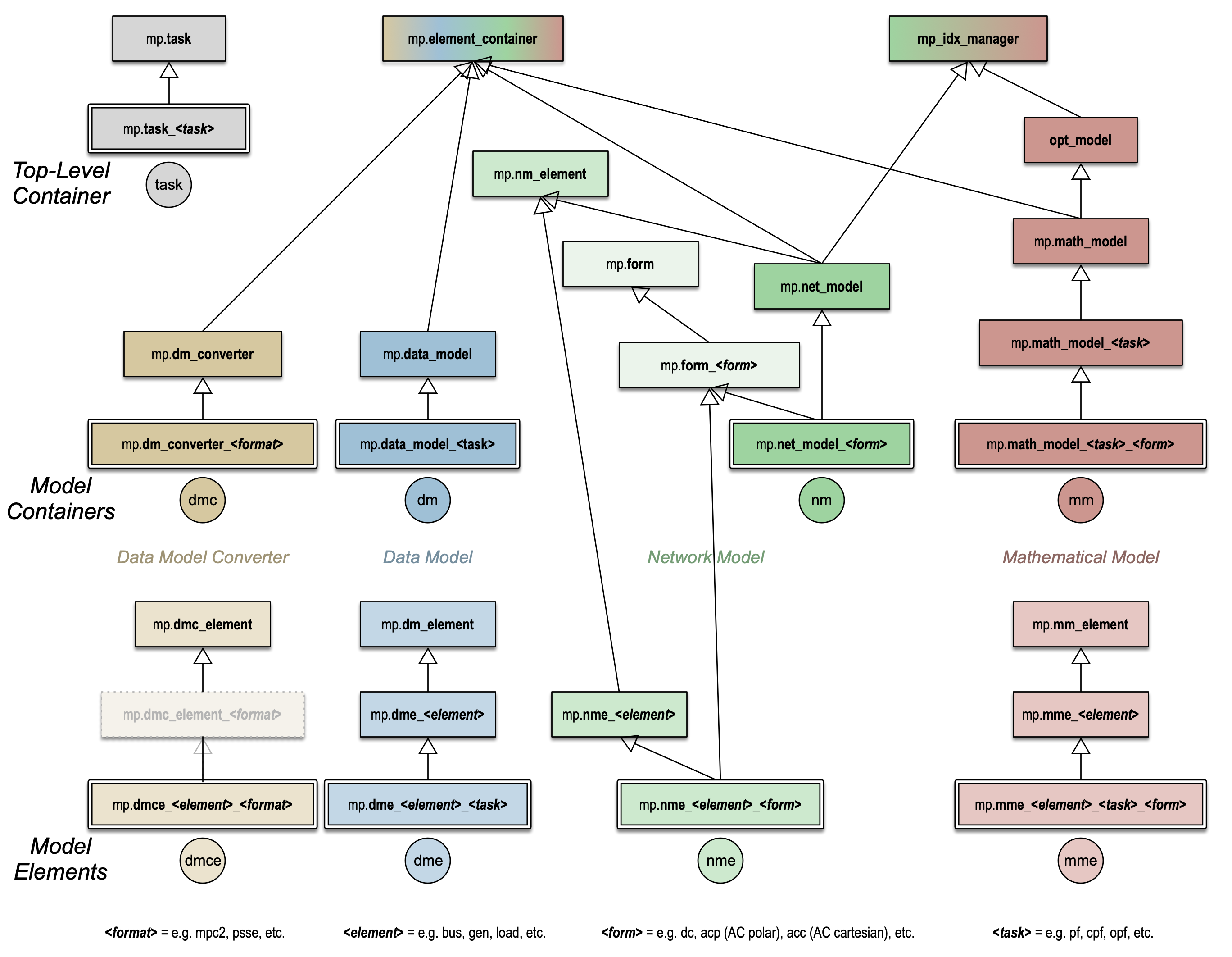
Figure 3.3 MATPOWER Class Hierarchies
Subclasses in these hierarchies are distinguished from one another by various attributes. For example, task classes are distinguished by the type of task or problem being solved (e.g. PF, CPF, OPF), data model converters by the data format (e.g. MATPOWER case v2, PSS/E RAW), data models by the task, network models by the formulation (e.g. DC, AC polar, AC cartesian), mathematical models by the task and formulation. That goes for both the container classes and their respective element classes, which are also distinguished by the corresponding element type (e.g. bus, generator, transmission line).
The mp.element_container is a mixin class providing shared functionality for the four container types mentioned above, implementing a set of elements, which can be addressed by both index and name and supplying the properties elements and element_classes.
Other mixin classes are also sometimes used when certain functionality and implementation is shared across classes in ways that do not match the primary inheritance paths.
3.3. Two MATPOWER Frameworks
MATPOWER currently provides two approaches to utilizing the object-oriented MATPOWER core architecture.
The first, which we call the legacy MATPOWER framework, wraps MP-Core objects inside the legacy user interface, with its inherent limitations, in order to provide backward compatibility for legacy user customization mechanisms. This allows MP-Core to be used internally to implement all of the legacy PF, CPF and OPF functionality and, even more importantly, to be validated by MATPOWER’s extensive legacy test suite.
The second approach, which we call the flexible MATPOWER framework, involves an object-oriented design with a new customization architecture, able to make the full scope of flexibility of MP-Core accessible to the end user. For example, this framework is required to take advantage of new modeling capabilities to add multiphase unbalanced and hybrid models. It provides its own version of the top-level user functions, namely run_pf(), run_cpf(), and run_opf() (note the underscores in the names).
One of the primary differences between the two frameworks is that the legacy framework converts the MATPOWER case data to internal format, removing offline equipment and renumbering buses consecutively using the legacy ext2int() function, before creating the task object and running it. After solving, it converts the case back to the external format using int2ext() before returning the result. This conversion is required for the legacy user callback mechanisms, but is not necessary for MP-Core itself, so it is not included in the flexible framework.
3.4. MATPOWER Customization
The primary motivation behind the design of MP-Core was to facilitate customization, both for the end user and for the developer who wants to add new capabilities to MATPOWER itself. Given the object-oriented architecture, this is possible by simply subclassing existing classes to modify or override their behavior or adding completely new classes, which can often inherit significant functionality from existing abstract base classes.
The flexible MATPOWER framework includes a mechanism for defining and using MATPOWER extensions (see Chapter 9.3). A MATPOWER extension is essentially a collection of modifications and additions to be made to the set default classes used to construct the task, model and model element objects.