How to Create a New Element Type
This guide demonstrates how to create a new element type. MATPOWER includes implementations of numerous standard element types such as buses, generators, loads, transmission lines, transformers, etc. For this discussion, we use a DC transmission line model, equivalent to the one described in Section 7.6.3 of the legacy MATPOWER User's Manual.
DC Transmission Line
The model used here for a DC transmission line is a 2-port model with a 2 non-voltage states. That is, each DC line connects to exactly 2 buses, and there are two additional complex states representing the complex power injections at the ports. In addition, each DC line is assumed to have an active power loss \(p_\mathrm{loss}\) that is a linear function of the active power \(p_1\) at the from bus.
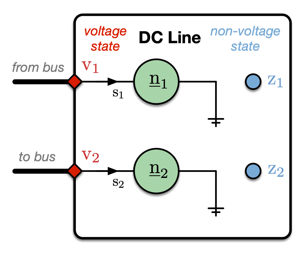
Figure 1 AC Model for DC Line
Figure 1 shows a diagram of the 2-port DC line, where the port power injections are given by the following equations,
In this case, the parameters \(\param{\cscal{n}}_1\) and \(\param{\cscal{n}}_2\) are both equal to 1. In addition, we have the following constraint on the active and reactive port power injections, where \(\cscal{s}_k = p_k + j q_k\).
For power flow problems, each of the connected buses can be specified as a PV bus, with specified voltage magnitude setpoint. For OPF problems, a cost may be applied to the from end active injection.
Creating a new element type involves defining and implmementing the corresponding classes for each layer (data, network, and mathematical) of modeling, as well as a corresponding data converter element for each data format. Each of these classes has a name() method that returns the same value, linking them to one another and together defining the DC line element type. That is, in each type of element class, you will see the following method defined.
function name = name(obj)
    name = 'legacy_dcline';
end
Data Model Element
We begin with the data model element, whose role and structure is described in Data Model Elements in the MATPOWER Developer’s Manual. This is where you define each piece of data that corresponds to the element. All elements include a unique identifier, a name, and a status flag. Most elements are connected to other elements (e.g. buses) and the connectivity data (e.g. IDs of connected buses) are included in the data model. Any device parameters, either physical or operational are also included, along with any input and/or solution values of the state of the element.
For each DC line, the data consists of the two buses to which its ports are connected, a status flag, active and reactive flows at each end, voltage set points at each end, upper and lower limits on the active and reactive injections, the two loss coefficients, and, for OPF problems, shadow prices on the injection bounds.
Since some pieces of data are only needed for the OPF, we define the base data model element for the DC line in the mp.dme_dcline class, and extend it via mp.dme_dcline_opf to include the data required for the OPF.
This data is stored in the main data table in the tab property of the data model element object of type mp.dme_dcline. This is a MATLAB table object, or an mp_table object if running in Octave. The names of the columns in tab are shown in Table 1 below. Each row in tab corresponds to an individual DC line, which means there is a single instance of a DC line data model element object to hold the data for all DC lines in the system.
Table 1 DC Line Data Model Column Names
Description
bus_fr,bus_tobus numbers for the from port (1) and to port (2) connections, respectively
loss0,loss1loss coefficient parameters \(\param{\cscal{l}}_0\) and \(\param{\cscal{l}}_1\), respectively
vm_setpoint_fr,vm_setpoint_tovoltage magnitude set points in p.u. for from and to buses, respectively
p_fr_lb,p_fr_ublower and upper bounds, \(\param{p}^\mathrm{min}_1\) and \(\param{p}^\mathrm{max}_1\), on active power injection at from bus (port 1)
q_fr_lb,q_fr_ublower and upper bounds, \(\param{q}^\mathrm{min}_1\) and \(\param{q}^\mathrm{max}_1\), on reactive power injection at from bus (port 1)
q_to_lb,q_to_ublower and upper bounds, \(\param{q}^\mathrm{min}_2\) and \(\param{q}^\mathrm{max}_1\), on reactive power injection at to bus (port 2)
p_fr,q_fractive and reactive injections, \(p_1\) and \(q_1\), at from port
p_to,q_toactive and reactive injections, \(p_2\) and \(q_2\), at to port
Listing 1 shows the source code for mp.dme_legacy_dcline. The first thing to notice is that, as with all data model element classes, it inherits from mp.dm_element. Please see the mp.dm_element reference documentation for an overview of the functionality provided and for more details on the methods overridden by mp.dme_legacy_dcline.
 1classdef dme_legacy_dcline < mp.dm_element
 2    properties
 3        fbus    % bus index vector for "from" port (port 1) (all DC lines)
 4        tbus    % bus index vector for "to" port (port 2) (all DC lines)
 5        fbus_on % vector of "from" bus indices into online buses (in-service DC lines)
 6        tbus_on % vector of "to" bus indices into online buses (in-service DC lines)
 7        loss0   % constant term of loss function (p.u.) (in-service DC lines)
 8        loss1   % linear coefficient of loss function (in-service DC lines)
 9        p_fr_start  % initial active power (p.u.) at "from" port (in-service DC lines)
10        p_to_start  % initial active power (p.u.) at "to" port (in-service DC lines)
11        q_fr_start  % initial reactive power (p.u.) at "from" port (in-service DC lines)
12        q_to_start  % initial reactive power (p.u.) at "to" port (in-service DC lines)
13        vm_setpoint_fr  % from bus voltage magnitude setpoint (p.u.) (in-service DC lines)
14        vm_setpoint_to  % to bus voltage magnitude setpoint (p.u.) (in-service DC lines)
15        p_fr_lb % p.u. lower bound on active power flow at "from" port (in-service DC lines)
16        p_fr_ub % p.u. upper bound on active power flow at "from" port (in-service DC lines)
17        q_fr_lb % p.u. lower bound on reactive power flow at "from" port (in-service DC lines)
18        q_fr_ub % p.u. upper bound on reactive power flow at "from" port (in-service DC lines)
19        q_to_lb % p.u. lower bound on reactive power flow at "to" port (in-service DC lines)
20        q_to_ub % p.u. upper bound on reactive power flow at "to" port (in-service DC lines)
21    end     %% properties
22
23    methods
24        function name = name(obj)
25            name = 'legacy_dcline';
26        end
27
28        % (other methods listed and described individually below)
29
30    end     %% methods
31end         %% classdef
For element types that connect to one or more buses, it is typical to define a property for each port in the data model element class. In our case, there are two properties, fbus and tbus, which will hold bus index vectors for ports 1 and 2, respectively. That is dme.tbus(k) will refer to the index of the bus connected to port 2, the to bus, of the DC line defined in row k of the data table.
Note
The contents of fbus and tbus are not bus IDs, that is external bus numbers, but rather internal indices of the corresponding buses, that is, row indices into dm.elements.bus.tab, the table of all buses in the bus data model element object.
The fbus_on and tbus_on properties, on the other, hand map in-service DC lines to the in-service buses. That is dme.fbus_on(k) is the index into the list of in-service buses for the bus connected to port 1, the from bus, of the k-th in-service DC line.
The other properties correspond to the respective columns in the data table, but after removing DC lines that are out-of-service and, in some cases, converting to per unit. Those that end in _start are for the initial value of the respective variable.
Naming
The name() method returns 'legacy_dcline', the name used internally for this element type. The label() and labels() methods provide strings to use for singular and plural user visible labels to use when displaying DC line elements.
function name = name(obj)
    name = 'legacy_dcline';
end

function label = label(obj)
    label = 'DC Line';
end

function label = labels(obj)
    label = 'DC Lines';
end
Connectivity
The cxn_type() and cxn_idx_prop() methods specify that 'legacy_dcline' objects connect to 'bus' objects, and that the corresponding bus indices for ports 1 and 2 can be found in properties fbus and tbus, respectively.
function name = cxn_type(obj)
    name = 'bus';
end

function name = cxn_idx_prop(obj)
    name = {'fbus', 'tbus'};
end
Main Data Table
The names of the columns in the DC line’s main data table are defined by the return value of main_table_var_names(). Note that it is important to call the parent method to include inherited column names, in particular, those common to all data model elements (i.e. 'uid', 'name', 'status', 'source_uid').
function names = main_table_var_names(obj)
    names = horzcat( main_table_var_names@mp.dm_element(obj), ...
        {'bus_fr', 'bus_to', 'loss0', 'loss1', ...
        'vm_setpoint_fr', 'vm_setpoint_to', ...
        'p_fr_lb', 'p_fr_ub', ...
        'q_fr_lb', 'q_fr_ub', 'q_to_lb', 'q_to_ub', ...
        'p_fr', 'q_fr', 'p_to', 'q_to'} );
end
Output Values
The export_vars() method returns the names of the columns in the table that should be exported back to the data source after solving. That is, it is the list of output columns whose values may have been updated by running the task. In this case, it only includes the active and reactive injections at the ports.
function vars = export_vars(obj)
    vars = {'p_fr', 'q_fr', 'p_to', 'q_to'};
end
The entries in the struct returned by export_vars_offline_val() specify values to assign to fields in out-of-service DC lines. Specifically, we set all of the active and reactive flows to 0 for DC lines that are out-of-service.
function s = export_vars_offline_val(obj)
    s = export_vars_offline_val@mp.dm_element(obj);     %% call parent
    s.p_fr = 0;
    s.q_fr = 0;
    s.p_to = 0;
    s.q_to = 0;
end
Building the Element in Stages
When a data model object and its elements are created, they are built in the stages described in Building a Data Model in the MATPOWER Developer’s Manual.
The initialize() method is called during the initialize stage. It takes advantage of the bus ID-to-index mapping available from the 'bus' data model element object to populate the fbus and tbus properties from the corresponding columns in the main data table.
function obj = initialize(obj, dm)
    initialize@mp.dm_element(obj, dm);  %% call parent

    %% get bus mapping info
    b2i = dm.elements.bus.ID2i;     %% bus num to idx mapping

    %% set bus index vectors for port connectivity
    obj.fbus = b2i(obj.tab.bus_fr);
    obj.tbus = b2i(obj.tab.bus_to);
end
The update_status() method, called during the update status stage, updates the default online/offline status, which has already been initialized from the status column of the main data table, to remove from service any DC line that is connected to an offline bus. After calling the parent method to populate the on and off properties, this method also updates some data in the bus data model element object to set the bus type for DC terminal buses to PV and turn on their voltage-controlled flag.
function obj = update_status(obj, dm)
    %

    %% get bus status info
    bus_dme = dm.elements.bus;
    bs = bus_dme.tab.status;    %% bus status

    %% update status of branches connected to isolated/offline buses
    obj.tab.status = obj.tab.status & bs(obj.fbus) & ...
                                      bs(obj.tbus);

    %% call parent to fill in on/off
    update_status@mp.dm_element(obj, dm);

    %% for all online DC lines ...
    %% ... set terminal buses (except ref) to PV type
    idx = [obj.fbus(obj.on); obj.tbus(obj.on)]; %% all terminal buses
    idx(bus_dme.type(idx) == mp.NODE_TYPE.REF) = [];    %% except ref
    bus_dme.set_bus_type_pv(dm, idx);

    %% set bus_dme.vm_control
    obj.fbus_on = bus_dme.i2on(obj.fbus(obj.on));
    obj.tbus_on = bus_dme.i2on(obj.tbus(obj.on));
    bus_dme.vm_control(obj.fbus_on) = 1;
    bus_dme.vm_control(obj.tbus_on) = 1;
end
Note that both initialize() and update_status() rely on the fact that the respective methods have already been called for 'bus' objects, before they are called for 'legacy_dcline' objects. The order corresponds to their order in dm.element_classes which is determined by the default, defined in the data model class, and any MATPOWER extensions or options used to modify that default.
By the time build_params() is called in the build parameters stage of the data model build, the global data model values, such as dm.base_mva, have already been loaded and the update status stage has completed, filling in the on property of the object. This allows us to populate the various properties of the object with parameters for online elements only. These are pulled from the object’s main data table in tab with per unit conversions applied where appropriate.
The final step in build_params() is a call to apply_vm_setpoints() which applies the specified voltage setpoints to the appropriate buses in the bus data model element object.
function obj = build_params(obj, dm)
    obj.loss0 = obj.tab.loss0(obj.on) / dm.base_mva;
    obj.loss1 = obj.tab.loss1(obj.on);
    obj.p_fr_start = obj.tab.p_fr(obj.on) / dm.base_mva;
    obj.p_to_start = (obj.loss1 - 1) .* obj.p_fr_start + obj.loss0;
    obj.q_fr_start = -obj.tab.q_fr(obj.on) / dm.base_mva;
    obj.q_to_start = -obj.tab.q_to(obj.on) / dm.base_mva;
    obj.vm_setpoint_fr = obj.tab.vm_setpoint_fr(obj.on);
    obj.vm_setpoint_to = obj.tab.vm_setpoint_to(obj.on);
    obj.p_fr_lb = obj.tab.p_fr_lb(obj.on) / dm.base_mva;
    obj.p_fr_ub = obj.tab.p_fr_ub(obj.on) / dm.base_mva;
    obj.q_fr_lb = obj.tab.q_fr_lb(obj.on) / dm.base_mva;
    obj.q_fr_ub = obj.tab.q_fr_ub(obj.on) / dm.base_mva;
    obj.q_to_lb = obj.tab.q_to_lb(obj.on) / dm.base_mva;
    obj.q_to_ub = obj.tab.q_to_ub(obj.on) / dm.base_mva;

    obj.apply_vm_setpoints(dm);
end

function obj = apply_vm_setpoints(obj, dm)
    bus_dme = dm.elements.bus;
    i_fr = find(bus_dme.vm_control(obj.fbus_on));
    i_to = find(bus_dme.vm_control(obj.tbus_on));
    bus_dme.vm_start(obj.fbus_on(i_fr)) = obj.vm_setpoint_fr(i_fr);
    bus_dme.vm_start(obj.tbus_on(i_to)) = obj.vm_setpoint_to(i_to);
end
Pretty Printing
The mp.dme_legacy_dcline class is also where you override any of the pretty-printing methods to implement DC line sections in the pretty-printed output.
The count (cnt) section is handled automatically by methods in the base class and there is no extremes (ext) section for DC lines, so no overrides are necessary for those sections.
For the summary (sum) section, pp_have_section_sum() indicates that the section is present for DC lines, and pp_data_sum() provides the content, printing the total active and reactive losses in a format consistent with the standard element types.
function TorF = pp_have_section_sum(obj, mpopt, pp_args)
    TorF = true;
end

function obj = pp_data_sum(obj, dm, rows, out_e, mpopt, fd, pp_args)
    %% call parent
    pp_data_sum@mp.dm_element(obj, dm, rows, out_e, mpopt, fd, pp_args);

    %% print DC line summary
    fprintf(fd, '  %-29s  %12.2f MW', 'Total DC line losses', ...
        sum(obj.tab.p_fr(obj.on)) - sum(obj.tab.p_to(obj.on)) );
    if mpopt.model(1) ~= 'D'    %% AC model
        fprintf(fd, ' %12.2f MVAr', ...
            sum(obj.tab.q_fr(obj.on)) + sum(obj.tab.q_to(obj.on)) );
    end
    fprintf(fd, '\n');
end
The details (det) section, which outputs the details for each individual DC line, is implemented by overriding pp_have_section_det(), pp_get_headers_det() and pp_data_det(). The first indicates that the section is present, the second returns a cell array of strings to use as header rows, and the third returns a string with the output for the k-th DC line.
function TorF = pp_have_section_det(obj, mpopt, pp_args)
    TorF = true;
end

function h = pp_get_headers_det(obj, dm, out_e, mpopt, pp_args)
    h = [ pp_get_headers_det@mp.dm_element(obj, dm, out_e, mpopt, pp_args) ...
        {   ' DC Line    From       To              Power Flow (MW)      Loss    Reactive Inj (MVAr)', ...
            '   ID      Bus ID    Bus ID   Status    From       To       (MW)      From       To', ...
            '--------  --------  --------  ------  --------  --------  --------  --------  --------' } ];
    %%       1234567 123456789 123456789 -----1 1234567.90 123456.89 123456.89 123456.89 123456.89
end

function str = pp_data_row_det(obj, dm, k, out_e, mpopt, fd, pp_args)
    str = sprintf('%7d %9d %9d %6d %10.2f %9.2f %9.2f %9.2f %9.2f', ...
        obj.tab.uid(k), obj.tab.bus_fr(k), obj.tab.bus_to(k), ...
        obj.tab.status(k), ...
        obj.tab.p_fr(k), obj.tab.p_to(k), ...
        obj.tab.p_fr(k) - obj.tab.p_to(k), ...
        obj.tab.q_fr(k), obj.tab.q_to(k) );
end
See lib/t/+mp/dme_legacy_dcline.m for the complete mp.dme_legacy_dcline source.
OPF Subclass
For OPF problems, there are a few additions to the data model element for DC lines, and we use a subclass of mp.dme_legacy_dcline. First, there are a few extra columns in the main data table for shadow prices on limits. Notice that these are also included as output values, which are zeroed out for out-of-service DC lines.
While we could have put the limit parameters themselves in the OPF subclass, since they are not explicitly used when running a simple power flow, we chose to keep them in the base class so the data is available for power flow and CPF in case the user would like to check the solutions against the limits or implement controls based on them.
 1classdef dme_legacy_dcline_opf < mp.dme_legacy_dcline
 2    methods
 3        function names = main_table_var_names(obj)
 4            names = horzcat( main_table_var_names@mp.dme_legacy_dcline(obj), ...
 5                {   'cost', ...
 6                    'mu_p_fr_lb', 'mu_p_fr_ub', ...
 7                    'mu_q_fr_lb', 'mu_q_fr_ub', ...
 8                    'mu_q_to_lb', 'mu_q_to_ub'  } );
 9        end
10
11        function vars = export_vars(obj)
12            vars = horzcat( export_vars@mp.dme_legacy_dcline(obj), ...
13                {   'vm_setpoint_fr', 'vm_setpoint_to', ...
14                    'mu_p_fr_lb', 'mu_p_fr_ub', ...
15                    'mu_q_fr_lb', 'mu_q_fr_ub', ...
16                    'mu_q_to_lb', 'mu_q_to_ub'  } );
17        end
18
19        function s = export_vars_offline_val(obj)
20            s = export_vars_offline_val@mp.dme_legacy_dcline(obj);  %% call parent
21            s.mu_p_fr_lb = 0;
22            s.mu_p_fr_ub = 0;
23            s.mu_q_fr_lb = 0;
24            s.mu_q_fr_ub = 0;
25            s.mu_q_to_lb = 0;
26            s.mu_q_to_ub = 0;
27        end
28
29        % (additional methods listed and described below)
30    end     %% methods
31end         %% classdef
The other addition in the OPF subclass is an optional cost on the active power flow in the DC line. This cost is specified in the same way as a generator cost, either as a set of polynomial coefficients, or as a set of breakpoints in a piecewise linear function. It appears as a column in the main table and is of type mp.cost_table.
There is also a have_cost() method that returns true for OPF subclass and false in the base class. It is used by the export routines of the data model converter element to determine whether or not to export cost data.
function TorF = have_cost(obj)
    TorF = 1;
end
The build_cost_params() method is called during the creation of an OPF mathematical model to extract the costs from the data and put it in a form more convenient for adding to the math model. The implementation is built on the same mp.cost_table and mp.cost_table_utils classes used for generator costs.
function cost = build_cost_params(obj, dm)
    if ismember('cost', obj.tab.Properties.VariableNames)
        poly = mp.cost_table_utils.poly_params(obj.tab.cost, obj.on, dm.base_mva);
        pwl = mp.cost_table_utils.pwl_params(obj.tab.cost, obj.on, dm.base_mva);

        cost = struct( ...
                'poly', poly, ...
                'pwl',  pwl ...
            );
    else
        cost = struct([]);
    end
end
Finally, there are several methods for handling the pretty-printing of the limits (lim) section, which is only relevant for the OPF. The pretty_print() method is overridden to set up some data for limit sections, namely flows and shadow prices, to be passed via pp_args to the methods that do the printing.
function obj = pretty_print(obj, dm, section, out_e, mpopt, fd, pp_args)
    switch section
        case 'lim'
            %% pass flows and limits to parent
            p_fr = obj.tab.p_fr;
            lb = obj.tab.p_fr_lb;
            ub = obj.tab.p_fr_ub;
            pp_args.legacy_dcline.flow = struct( 'p_fr', p_fr, ...
                                                 'lb', lb, ...
                                                 'ub', ub );
    end

    pretty_print@mp.dme_legacy_dcline(obj, dm, section, out_e, mpopt, fd, pp_args);
end
The pp_have_section_lim() method indicates that DC lines do have a limits section, pp_binding_rows_lim() returns the indices of the DC lines with binding limits, pp_get_headers_lim() returns a cell array of char arrays for the header lines, and pp_data_row_lim() returns a char array displaying the limit data for DC line k.
function TorF = pp_have_section_lim(obj, mpopt, pp_args)
    TorF = true;
end

function rows = pp_binding_rows_lim(obj, dm, out_e, mpopt, pp_args)
    flow = pp_args.legacy_dcline.flow;
    rows = find( obj.tab.status & ( ...
                flow.p_fr < flow.lb + obj.ctol | ...
                flow.p_fr > flow.ub - obj.ctol | ...
                obj.tab.mu_p_fr_lb > obj.ptol | ...
                obj.tab.mu_p_fr_ub > obj.ptol ));
end

function h = pp_get_headers_lim(obj, dm, out_e, mpopt, pp_args)
    h = [ pp_get_headers_lim@mp.dme_shared_opf(obj, dm, out_e, mpopt, pp_args) ...
        {   ' DC Line    From       To                   Active Power Flow (MW)', ...
            '   ID      Bus ID    Bus ID     mu LB       LB      p_fr      UB      mu UB', ...
            '--------  --------  --------  ---------  -------  -------  -------  ---------' } ];
    %%       1234567 123456789 123456789 123456.890 12345.78 12345.78 12345.78 123456.890
end

function str = pp_data_row_lim(obj, dm, k, out_e, mpopt, fd, pp_args)
    flow = pp_args.legacy_dcline.flow;

    if (flow.p_fr(k) < flow.lb(k) + obj.ctol || ...
            obj.tab.mu_p_fr_lb(k) > obj.ptol)
        mu_lb = sprintf('%10.3f', obj.tab.mu_p_fr_lb(k));
    else
        mu_lb = '      -   ';
    end
    if (flow.p_fr(k) > flow.ub(k) - obj.ctol || ...
            obj.tab.mu_p_fr_ub(k) > obj.ptol)
        mu_ub = sprintf('%10.3f', obj.tab.mu_p_fr_ub(k));
    else
        mu_ub = '      -   ';
    end

    str = sprintf('%7d %9d %9d %10s %8.2f %8.2f %8.2f %10s', ...
        obj.tab.uid(k), obj.tab.bus_fr(k), obj.tab.bus_to(k), ...
        mu_lb, flow.lb(k), flow.p_fr(k), flow.ub(k), mu_ub);
end
See lib/t/+mp/dme_legacy_dcline_opf.m for the complete mp.dme_legacy_dcline_opf source.
Data Model Converter Element
The role of the data model converter element, as described in Data Model Converter Elements in MATPOWER Developer’s Manual, is to implement the functionality needed to import and export data from a specific external format. In this case, we need to import from and export to the dcline and dclinecost fields in a MATPOWER case struct (v2) format.
There is a single class, mp.dmce_legacy_dcline_mpc2 to implement this functionality. As with all data model converter elements, it inherits from mp.dmc_element and defines a name() method.
 1classdef dmce_legacy_dcline_mpc2 < mp.dmc_element
 2    methods
 3        function name = name(obj)
 4            name = 'legacy_dcline';
 5        end
 6
 7        % (other methods listed and described individually below)
 8
 9    end     %% methods
10end         %% classdef
Main Field in Data Source
Generally, the main data table in the data model element corresponds to a particular field in the data source (the MATPOWER case struct, i.e. mpc).
The name of this field is defined by the return value of data_field().
function df = data_field(obj)
    df = 'dcline';
end
When exporting to a new MATPOWER case struct, the default_export_data_table() method is called to initialize the value of this field, i.e. of mpc.dcline. In this case, it is simply a matrix of all zeros with the expected number of rows and columns. The number of rows is retrieved from the export specification by the default_export_data_nrows() method.
function dt = default_export_data_table(obj, spec)
    %% define named indices into data matrices
    c = idx_dcline;

    nr = obj.default_export_data_nrows(spec);
    dt = zeros(nr, c.QMAXT);
end
Table Variable Map
The majority of the functionality of the data model converter element is handled by the table_var_map() method. This method returns a variable map struct as summarized in Table 6.1 in the MATPOWER Developer’s Manual. This map defines where to get the data for each variable in the data model element’s main data table. For our DC line, this is the data listed in Table 1.
Most of the variables are simply copied directy from/to the corresponding column in mpc.dcline. In this case, the corresponding entry in the the map is a cell array whose first element has already been initialized to 'col' by the parent method, so we simply set the second element to the index of the corresponding column. For example, the active power flow in dme.tab.p_fr is copied directly from/to mpc.dcline(:, c.PF) (i.e. column 4). The uid field specifies that the uid variable be assigned consecutive integer IDs, starting at 1, and the name and source_uid variables are simply assigned a cell array of empty char arrays.
The only other variable not pulled directly from a column of mpc.dcline is the cost variable. This comes from mpc.dclinecost and the variable map entry specifies custom import and export methods described below to handle the import/export directly.
function vmap = table_var_map(obj, dme, mpc)
    vmap = table_var_map@mp.dmc_element(obj, dme, mpc);

    %% define named indices into data matrices
    c = idx_dcline;

    gcip_fcn = @(ob, mpc, spec, vn)dcline_cost_import(ob, mpc, spec, vn);
    gcep_fcn = @(ob, dme, mpc, spec, vn, ridx)dcline_cost_export(ob, dme, mpc, spec, vn, ridx);

    %% mapping for each name, default is {'col', []}
    vmap.uid                = {'IDs'};      %% consecutive IDs, starting at 1
    vmap.name               = {'cell', ''};     %% empty char
    vmap.status{2}          = c.BR_STATUS;
    vmap.source_uid         = {'cell', ''};     %% empty char
    vmap.bus_fr{2}          = c.F_BUS;
    vmap.bus_to{2}          = c.T_BUS;
    vmap.loss0{2}           = c.LOSS0;
    vmap.loss1{2}           = c.LOSS1;
    vmap.vm_setpoint_fr{2}  = c.VF;
    vmap.vm_setpoint_to{2}  = c.VT;
    vmap.p_fr_lb{2}         = c.PMIN;
    vmap.p_fr_ub{2}         = c.PMAX;
    vmap.q_fr_lb{2}         = c.QMINF;
    vmap.q_fr_ub{2}         = c.QMAXF;
    vmap.q_to_lb{2}         = c.QMINT;
    vmap.q_to_ub{2}         = c.QMAXT;
    vmap.p_fr{2}            = c.PF;
    vmap.q_fr{2}            = c.QF;
    vmap.p_to{2}            = c.PT;
    vmap.q_to{2}            = c.QT;
    if isfield(vmap, 'cost')
        vmap.cost        = {'fcn', gcip_fcn, gcep_fcn};
        vmap.mu_p_fr_lb{2}  = c.MU_PMIN;
        vmap.mu_p_fr_ub{2}  = c.MU_PMAX;
        vmap.mu_q_fr_lb{2}  = c.MU_QMINF;
        vmap.mu_q_fr_ub{2}  = c.MU_QMAXF;
        vmap.mu_q_to_lb{2}  = c.MU_QMINT;
        vmap.mu_q_to_ub{2}  = c.MU_QMAXT;
    end
end
Custom Import/Export Functions
Finally, the custom import and export methods for the DC line cost work explicitly with mpc.dclinecost using some static methods from mp.dmce_gen_mpc2 to convert from/to the legacy gencost format.
function val = dcline_cost_import(obj, mpc, spec, vn)
    if isfield(mpc, 'dclinecost') && spec.nr
        val = mp.dmce_gen_mpc2.gencost2cost_table(mpc.dclinecost);
    else
        val = [];
    end
end

function mpc = dcline_cost_export(obj, dme, mpc, spec, vn, ridx)
    if dme.have_cost()
        cost = mp.dmce_gen_mpc2.cost_table2gencost( ...
                    [], dme.tab.cost, ridx);
        mpc.dclinecost(1:spec.nr, 1:size(cost, 2)) = cost;
    end
end
See lib/t/+mp/dmce_legacy_dcline_mpc2.m for the complete mp.dmce_legacy_dcline_mpc2 source.
Network Model Element
Next we define the DC line network model. Let’s assume we want implementations for a DC model as well as both polar and cartesian voltage formulations of the AC model. Because network models are formulation-specific, we define a class hierarchy for the network model element.
All Formulations
All DC line network model elements will inherit from mp.nme_legacy_dcline, shown in Listing 4, which in turn inherits from mp.nm_element. Please see the mp.nm_element reference documentation for an overview of the functionality provided and for more details on the methods overridden by mp.nme_legacy_dcline and its subclasses.
 1classdef (Abstract) nme_legacy_dcline < mp.nm_element
 2    methods
 3        function name = name(obj)
 4            name = 'legacy_dcline';
 5        end
 6
 7        function np = np(obj)
 8            np = 2;     %% this is a 2 port element
 9        end
10
11        function nz = nz(obj)
12            nz = 2;     %% 2 (possibly complex) non-voltage state per element
13        end
14    end     %% methods
15end         %% classdef
Once again, name() returns the name used internally for this element type, while the np() and nz() methods return the number of ports and non-voltage states, respectively. These are shared by all formulations.
AC Formulations
Anything that applies to both AC formulations, but not the DC formulation, is included in the abstract class mp.nme_legacy_dcline_ac, shown in Listing 5, which is a subclass of mp.nme_legacy_dcline. Any concrete network model element class that inherits from mp.nme_legacy_dcline_ac is also expected to be a subclass of a formulation class that inherits from mp.form_ac.
 1classdef (Abstract) nme_legacy_dcline_ac < mp.nme_legacy_dcline & mp.form_ac
 2    methods
 3        function obj = add_zvars(obj, nm, dm, idx)
 4            ndc = obj.nk;
 5            dme = obj.data_model_element(dm);
 6            switch idx{1}
 7                case 1      % flow at "from"
 8                    nm.add_var('zr', 'Pdcf', ndc, dme.p_fr_start, dme.p_fr_lb, dme.p_fr_ub);
 9                    nm.add_var('zi', 'Qdcf', ndc, dme.q_fr_start, dme.q_fr_lb, dme.q_fr_ub);
10                case 2      % flow at "to"
11                    nm.add_var('zr', 'Pdct', ndc, dme.p_to_start, -Inf, Inf);
12                    nm.add_var('zi', 'Qdct', ndc, dme.q_to_start, dme.q_to_lb, dme.q_to_ub);
13            end
14        end
15
16        function obj = build_params(obj, nm, dm)
17            build_params@mp.nme_legacy_dcline(obj, nm, dm); %% call parent
18            obj.N = speye(obj.nk * obj.nz);
19        end
20    end     %% methods
21end         %% classdef
The first method defined by mp.nme_legacy_dcline_ac, namely add_zvars(), adds variables for the real and imaginary parts of the non-voltage state variables, \(\cvec{z}_1\) and \(\cvec{z}_2\), to the network model, constructing the initial values from the appropriate columns in the data table, and including predefined bounds. Note that the variable named Pdcf is vector containing the real part of \(\cscal{z}_1\) for all DC lines in the network. Because the voltage variable representation is different for cartesian and polar formulations, the implementation of add_vvars() is deferred to the formulation-specific subclasses below.
The second method, build_params(), first calls its parent to build the incidence matrices C and D, then constructs the standard AC model parameters from the data model. The AC model and its parameters are described in AC Formulations in the MATPOWER Developer’s Manual.
Recall that, if we omit the arbitrary nonlinear injection components, \(\Snln(\X)\) or \(\Inln(\X)\), the standard AC network model for any element type can be defined in terms of the six parameters in the equations below, namely \(\YY\), \(\LL\), \(\MM\), \(\NN\), \(\iv\), and \(\sv\).
For a single DC line, based on Figure 1 and equation (58), all of these parameters are zero (with proper dimensions) except \(\NN\), which is a \(2 \times 2\) identity matrix.
However, build_params() must build stacked versions of these matrix and vector parameters that include all \(n_k\) DC lines in the system. In general, for matrix parameters, such as \(\NN\), the stacking is done such that each scalar element is replaced by a corresponding \(n_k \times n_k\) diagonal matrix. For the vector parameters, each scalar element becomes an \(n_k \times 1\) vector. In our case, we have only \(\NN\), and the stacked version is simply a \(2 n_k \times 2 n_k\) identiy matrix.
AC Cartesian vs Polar Formulations
Once the parameters have been built, all of the differences between the cartesian and polar voltage formulations are handled automatically by inheriting from the appropriate formulation class. For the cartesian voltage formulation, we use mp.nme_legacy_dcline_acc which inherits from mp.nme_legacy_dcline_ac and mp.form_acc.
1classdef nme_legacy_dcline_acc < mp.nme_legacy_dcline_ac & mp.form_acc
2end
For the polar voltage formulation, we use mp.nme_legacy_dcline_acp which inherits from mp.nme_legacy_dcline_ac and mp.form_acp.
1classdef nme_legacy_dcline_acp < mp.nme_legacy_dcline_ac & mp.form_acp
2end
DC Formulation
The implementation for the DC version is similar. The nme_legacy_dcline_dc class, shown in Listing 8, inherits from both mp.nme_legacy_dcline and mp.form_dc.
 1classdef nme_legacy_dcline_dc < mp.nme_legacy_dcline & mp.form_dc
 2    methods
 3        function obj = add_zvars(obj, nm, dm, idx)
 4            ndc = obj.nk;
 5            dme = obj.data_model_element(dm);
 6            switch idx{1}
 7                case 1      % flow at "from"
 8                    nm.add_var('z', 'Pdcf', ndc, dme.p_fr_start, dme.p_fr_lb, dme.p_fr_ub);
 9                case 2      % flow at "to"
10                    nm.add_var('z', 'Pdct', ndc, dme.p_to_start, -Inf, Inf);
11            end
12        end
13
14        function obj = build_params(obj, nm, dm)
15            build_params@mp.nme_legacy_dcline(obj, nm, dm); %% call parent
16            obj.K = speye(obj.nk * obj.nz);
17        end
18    end     %% methods
19end         %% classdef
It also overrides add_zvars() to add a set of named variables for each of the two non-voltage states, namely the active power flows at the “from” and “to” ends of the DC lines. In this case, the states \(z_1\) and \(z_2\) are real, so there are only two variables instead of four.
The build_params() method once again calls its parent to build the incidence matrices C and D, then constructs the standard DC model parameters from the data model. The DC model and its parameters are described in DC Formulation in the MATPOWER Developer’s Manual.
Recall that the standard DC network model for any element type can be defined in terms of the three parameters in the equation below, namely \(\BB\), \(\KK\), and \(\pv\).
For DC lines, the only one we need to define is the \(\KK\) matrix and, analogous to \(\NN\) in the AC formulation, it also is a \(2 n_k \times 2 n_k\) identiy matrix.
The complete source for the DC line network model element classes above can be found in:
Mathematical Model Element
The mathematical model base classes automatically handle adding variables defined by the ports and states in the network model and incorporating the nodal injections implied by the network model parameters defined by each element.
However, the mathematical model element can be used to add any additional variables, beyond the voltage and non-voltage state variable, and any additional constraints or costs.
It is also responsible for passing solution data back to the data model. A mathematical model is specific to both a task (PF, CPF, OPF) and a formulation. So once again, we define a hierarchy of classes.
All Tasks and Formulations
All math model elements for DC lines inherit from mp.mme_legacy_dcline, which defines only the name() method.
1classdef (Abstract) mme_legacy_dcline < mp.mm_element
2    methods
3        function name = name(obj)
4            name = 'legacy_dcline';
5        end
6    end     %% methods
7end         %% classdef
Power Flow
Since the DC line flows are not dispatchable for the power flow problem, the active power injections are fixed, so there is no need for any additional constraints to be added to the problem. The only role of the math model element in this case is to update the data model after the model has been solved. For this we override the data_model_update_on() method, which updates values for the in-service DC lines. Since the AC and DC power flow versions are slightly different, we have separate subclasses for each. In each case, the solved values of the network port injections are used to update the corresponding variables in the main data table.
 1classdef mme_legacy_dcline_pf_ac < mp.mme_legacy_dcline
 2    methods
 3        function obj = data_model_update_on(obj, mm, nm, dm, mpopt)
 4            %% legacy DC line active power
 5            pp = nm.get_idx('port');
 6            s_fr = nm.soln.gs_(pp.i1.legacy_dcline(1):pp.iN.legacy_dcline(1));
 7            s_to = nm.soln.gs_(pp.i1.legacy_dcline(2):pp.iN.legacy_dcline(2));
 8
 9            %% update in the data model
10            dme = obj.data_model_element(dm);
11            dme.tab.p_fr(dme.on) = real(s_fr) * dm.base_mva;
12            dme.tab.q_fr(dme.on) = -imag(s_fr) * dm.base_mva;
13            dme.tab.p_to(dme.on) = -real(s_to) * dm.base_mva;
14            dme.tab.q_to(dme.on) = -imag(s_to) * dm.base_mva;
15        end
16    end     %% methods
17end         %% classdef
 1classdef mme_legacy_dcline_pf_dc < mp.mme_legacy_dcline
 2    methods
 3        function obj = data_model_update_on(obj, mm, nm, dm, mpopt)
 4            %% legacy DC line active power
 5            pp = nm.get_idx('port');
 6            p_fr = nm.soln.gp(pp.i1.legacy_dcline(1):pp.iN.legacy_dcline(1));
 7            p_to = nm.soln.gp(pp.i1.legacy_dcline(2):pp.iN.legacy_dcline(2));
 8
 9            %% update in the data model
10            dme = obj.data_model_element(dm);
11            dme.tab.p_fr(dme.on) = p_fr * dm.base_mva;
12            dme.tab.q_fr(dme.on) = 0;
13            dme.tab.p_to(dme.on) = -p_to * dm.base_mva;
14            dme.tab.q_to(dme.on) = 0;
15        end
16    end     %% methods
17end         %% classdef
Optimal Power Flow
For the OPF, there are a number of additions, including the constraint on the “from” and “to” end flows from (59) and any cost on the flow, which could be polynomial or piecewise linear. All of these are identical for AC and DC formulations, so we implement them in a class mp.mme_legacy_dcline_opf that will serve as a parent for both formulations.
 1classdef (Abstract) mme_legacy_dcline_opf < mp.mme_legacy_dcline
 2    properties
 3        cost
 4    end
 5
 6    methods
 7
 8        % (listed and described individually below)
 9
10    end     %% methods
11end         %% classdef
This class adds a cost property which holds the necessary cost data in a form that is convenient for constructing the math model costs. This field is populated by the build_cost_params() method by calling a method of the same name in the corresponding data model element.
function build_cost_params(obj, dm)
    dme = obj.data_model_element(dm);
    obj.cost = dme.build_cost_params(dm);
end
Any piecewise linear costs included in the cost data are implemented using a constrained cost variable (CCV) approach, just as with generator costs. This means we need to add cost variables and a set of linear constraints for each of these elements. First, we add an add_vars() method which first builds the cost data from the data model, then adds a variable named ydc to the math model, with dimenion equal to the number of piecewise linear costs.
function obj = add_vars(obj, mm, nm, dm, mpopt)
    %% collect/construct all legacy DC line cost parameters
    obj.build_cost_params(dm);

    %% piecewise linear costs
    if ~isempty(obj.cost) && obj.cost.pwl.n
        mm.add_var('ydc', obj.cost.pwl.n);
    end
end
We also override add_constraints() to add both the constraint for (59), a linear equality constrain on the Pdcf and Pdct optimization variables, as well as the constraints for any piecewise linear costs, which involve Pdcf and ydc.
function obj = add_constraints(obj, mm, nm, dm, mpopt)
    %% add constraint on active flows and ends of DC line
    dme = obj.data_model_element(dm);
    A = [spdiags(dme.loss1 - 1, 0, dme.n, dme.n) -speye(dme.n, dme.n)];
    b = -dme.loss0;
    mm.add_lin_constraint('dcline_legacy', A, b, b, {'Pdcf', 'Pdct'});

    %% piecewise linear costs
    if ~isempty(obj.cost) && obj.cost.pwl.n
        mm.add_lin_constraint('ycondc', obj.cost.pwl.A, [], obj.cost.pwl.b, {'Pdcf', 'ydc'});
    end
end
The add_costs() method adds the costs to the math model. As with generators, there are three kinds, polynomial costs of order less than 3, added as quadratic costs, polynomial costs of order 3 or greater, added as general nonlinear costs, and piecewise linear costs, added as simple linear costs on the ydc optimization variables we added for this purpose.
function obj = add_costs(obj, mm, nm, dm, mpopt)
    if ~isempty(obj.cost)
        %% (quadratic) polynomial costs on Pdcf
        if obj.cost.poly.have_quad_cost
            mm.add_quad_cost('polPdcf', obj.cost.poly.Q, obj.cost.poly.c, obj.cost.poly.k, {'Pdcf'});
        end

        %% (order 3 and higher) polynomial costs on Pg
        if ~isempty(obj.cost.poly.i3)
            dme = obj.data_model_element(dm);
            cost_Pdcf = @(xx)mp.cost_table.poly_cost_fcn( ...
                xx, dm.base_mva, dme.tab.cost.poly_coef(dme.on, :), ...
                obj.cost.poly.i3);
            mm.add_nln_cost('polPdcf', 1, cost_Pdcf, {'Pdcf'});
        end

        %% piecewise linear costs
        if obj.cost.pwl.n
            mm.add_quad_cost('pwldc', [], ones(obj.cost.pwl.n, 1), 0, {'ydc'});
        end
    end
end
Finally, a math model element for the OPF can provide an initial starting point for any variables it adds. This is implemented using the interior_x0 method.
function x0 = interior_x0(obj, mm, nm, dm, x0)
    %% set gen cost variables to something feasible
    if ~isempty(obj.cost) && obj.cost.pwl.n > 0
        vv = mm.get_idx();
        dme = obj.data_model_element(dm);
        maxc = max_pwl_cost(dme.tab.cost);
        x0(vv.i1.ydc:vv.iN.ydc) = maxc + 0.1 * abs(maxc);
    end
end
Data Model Update
As with the power flow, the updating of the data model is different for the AC and DC formulations, so we have two concrete classes for OPF, both of which override the data_model_update_on method.
In each case, as with the power flow, the flows are pulled from the values of the network port injections. The various constraint shadow prices, on the other hand, are pulled from the mathmatical model solution multipliers on the appropriate variable limits.
AC Optimal Power Flow
In the AC case, the voltage setpoints at the ends of DC lines are pulled from the network model node voltages multiplied by the appropriate incidence matrices to map them to the corresponding DC lines.
 1classdef mme_legacy_dcline_opf_ac < mp.mme_legacy_dcline_opf
 2    methods
 3        function obj = data_model_update_on(obj, mm, nm, dm, mpopt)
 4            dme = obj.data_model_element(dm);
 5            nme = obj.network_model_element(nm);
 6
 7            %% legacy DC line active power
 8            pp = nm.get_idx('port');
 9            s_fr = nm.soln.gs_(pp.i1.legacy_dcline(1):pp.iN.legacy_dcline(1));
10            s_to = nm.soln.gs_(pp.i1.legacy_dcline(2):pp.iN.legacy_dcline(2));
11            vm_setpoint = abs(nme.C' * nm.soln.v);
12
13            %% shadow prices on legacy DC line limits
14            vv = mm.get_idx();
15            lambda = mm.soln.lambda;
16            mu_p_fr_lb = lambda.lower(vv.i1.Pdcf:vv.iN.Pdcf);
17            mu_p_fr_ub = lambda.upper(vv.i1.Pdcf:vv.iN.Pdcf);
18            mu_q_fr_lb = lambda.lower(vv.i1.Qdcf:vv.iN.Qdcf);
19            mu_q_fr_ub = lambda.upper(vv.i1.Qdcf:vv.iN.Qdcf);
20            mu_q_to_lb = lambda.lower(vv.i1.Qdct:vv.iN.Qdct);
21            mu_q_to_ub = lambda.upper(vv.i1.Qdct:vv.iN.Qdct);
22
23            %% update in the data model
24            dme.tab.p_fr(dme.on) = real(s_fr) * dm.base_mva;
25            dme.tab.q_fr(dme.on) = -imag(s_fr) * dm.base_mva;
26            dme.tab.p_to(dme.on) = -real(s_to) * dm.base_mva;
27            dme.tab.q_to(dme.on) = -imag(s_to) * dm.base_mva;
28            dme.tab.vm_setpoint_fr(dme.on) = vm_setpoint(1:dme.n);
29            dme.tab.vm_setpoint_to(dme.on) = vm_setpoint(dme.n+1:end);
30            dme.tab.mu_p_fr_lb(dme.on) = mu_p_fr_lb / dm.base_mva;
31            dme.tab.mu_p_fr_ub(dme.on) = mu_p_fr_ub / dm.base_mva;
32            %% because of sign swap on reactive quantities, bounds are swapped
33            dme.tab.mu_q_fr_lb(dme.on) = mu_q_fr_ub / dm.base_mva;
34            dme.tab.mu_q_fr_ub(dme.on) = mu_q_fr_lb / dm.base_mva;
35            dme.tab.mu_q_to_lb(dme.on) = mu_q_to_ub / dm.base_mva;
36            dme.tab.mu_q_to_ub(dme.on) = mu_q_to_lb / dm.base_mva;
37        end
38    end     %% methods
39end         %% classdef
DC Optimal Power Flow
 1classdef mme_legacy_dcline_opf_dc < mp.mme_legacy_dcline_opf
 2    methods
 3        function obj = data_model_update_on(obj, mm, nm, dm, mpopt)
 4            dme = obj.data_model_element(dm);
 5
 6            %% legacy DC line active power
 7            pp = nm.get_idx('port');
 8            p_fr = nm.soln.gp(pp.i1.legacy_dcline(1):pp.iN.legacy_dcline(1));
 9            p_to = nm.soln.gp(pp.i1.legacy_dcline(2):pp.iN.legacy_dcline(2));
10
11            %% shadow prices on legacy DC line limits
12            vv = mm.get_idx();
13            lambda = mm.soln.lambda;
14            mu_p_fr_lb = lambda.lower(vv.i1.Pdcf:vv.iN.Pdcf);
15            mu_p_fr_ub = lambda.upper(vv.i1.Pdcf:vv.iN.Pdcf);
16
17            %% update in the data model
18            dme.tab.p_fr(dme.on) = p_fr * dm.base_mva;
19            dme.tab.q_fr(dme.on) = 0;
20            dme.tab.p_to(dme.on) = -p_to * dm.base_mva;
21            dme.tab.q_to(dme.on) = 0;
22            dme.tab.mu_p_fr_lb(dme.on) = mu_p_fr_lb / dm.base_mva;
23            dme.tab.mu_p_fr_ub(dme.on) = mu_p_fr_ub / dm.base_mva;
24        end
25    end     %% methods
26end         %% classdef
The complete source for the DC line mathematical model element classes above can be found in:
Using the New Element
Now that each of the element classes for the DC line have been implemented for each of the model layers and the data model converter, these classes need to be included when running a power flow, continuation power flow, or optimal power flow. If this implementation for DC lines were to be added to the set of standard elements, along side of buses, branches, and generators, for example, then the classes would be added to the lists assigned to the element_classes property in the constructor of the appropriate model container class. E.g. mp.nme_legacy_dcline_dc in mp.net_model_dc, and mp.mme_legacy_opf_dcline_ac in mp.math_model_opf_acc and mp.math_model_opf_acp.
However, for user additions that are not being contributed for inclusion in the standard MATPOWER distribution, the original MATPOWER source need not, and should not, be modified. Instead, we use the MATPOWER Extension API.
The How to Create an Extension guide explains how to package the DC line classes into an easy-to-use MATPOWER extension mp.xt_legacy_dcline, that can be used directly by run_pf(), run_cpf(), and run_opf(), as shown in the example below.
run_opf('t_case9_dcline', mpopt, 'mpx', mp.xt_legacy_dcline);
Go to How to Create an Extension.