How to Add an OPF Constraint
This guide describes how to add a nonlinear constraint to an optimal power flow using the flexible MATPOWER framework. For this example, we will implement an additional “oval-shaped” PQ capability curve for all generators as shown in Figure 3.
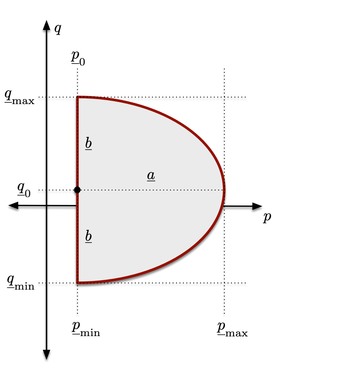
Figure 3 Oval PQ Capability Curve
That is, we add the following constraint on the active power \(p\) and reactive power \(q\) injected by each generator.
The parameters \(\param{p}_0\), \(\param{q}_0\), \(\param{a}\), and \(\param{b}\) are defined in terms of the active and reactive lower and upper bounds.
Adding this constraint affects only the mathematical model, with no changes to the data or network model layers. And since it relates only to generators, the implementation belongs in a math model element class for generators. Given that it is only relevant for AC OPF problems, we will override the mp.mme_gen_opf_ac with a new subclass mp.mme_gen_opf_ac_oval.
As the constraint is nonlinear, we will need to provide functions or methods to evaluate the constraint function and its first and second derivatives.
Function and Derivatives
If we use \(\rvec{p}\) and \(\rvec{q}\) to represent the vectors of active and reactive powers for all generators, and similarly for the parameters \(\param{\rvec{p}}_0\), \(\param{\rvec{q}}_0\), \(\param{\rvec{a}}\), and \(\param{\rvec{b}}\), we can write the full vector constraint function as follows, using the notation from Notation.
The first derivatives are
And the second derivatives are
Implementation
As mentioned above, the implementation will take the form of a new subclass, mp.mme_gen_opf_ac_oval, of the existing mp.mme_gen_opf_ac class.
classdef mme_gen_opf_ac_oval < mp.mme_gen_opf_ac
    methods
        % (defined below)
    end
end
We will be using the add_nln_constraint() method of the mathematical model object to add the constraints to the model, but first we must define the two methods that evaluate the constraints and derivatives. Since we will specify only the generators’ active and reactive injection variables as inputs, they will be passed to these functions as the cell array xx, with the vector of active powers in the first element and reactive powers in the second. Furthermore, these methods are implemented to allow the constraints to be evaluated for some subset of all generators, indexed by a vector idx.
The first method evaluates the constraint function and, optionally, its Jacobian, that is (75)–(77).
function [h, dh] = oval_pq_capability_fcn(obj, xx, idx, p0, q0, a2, b2)
    [p, q] = deal(xx{:});
    ng = length(p);
    if ~isempty(idx)
        p = p(idx);
        q = q(idx);
    end

    %% evaluate constraint function
    h = (p - p0).^2 ./ a2 + (q - q0).^2 ./ b2 - 1;

    %% evaluate constraint Jacobian
    if nargout > 1
        dhdp = spdiags(2*(p - p0) ./ a2, 0, ng, ng);
        dhdq = spdiags(2*(q - q0) ./ b2, 0, ng, ng);
        dh = [dhdp dhdq];
    end
end
The second evaluates the Hessian terms (78)–(81).
function d2H = oval_pq_capability_hess(obj, xx, lam, idx, p0, q0, a2, b2)
    [p, q] = deal(xx{:});
    if ~isempty(idx)
        p = p(idx);
        q = q(idx);
    end
    ng = length(p);
    zz = sparse(ng, ng);

    %% evaluate constraint Hessian
    d2H_pp = sparse(1:ng, 1:ng, 2 * lam ./ a2, ng, ng);
    d2H_qq = sparse(1:ng, 1:ng, 2 * lam ./ b2, ng, ng);
    d2H = [ d2H_pp  zz;
            zz      d2H_qq ];
end
Now we override the add_constraints() method to set up the parameters needed for the methods above, and to add the constraints to the model. The constraints are added as a set of nonlinear constraints named 'PQoval', defined as functions of the optimization variables named 'Pg' and 'Qg'.
function obj = add_constraints(obj, mm, nm, dm, mpopt)
    dme = obj.data_model_element(dm);

    %% generator PQ capability curve constraints
    idx = [];       %% which generators get this constraint
                    %% empty ==> all
    if isempty(idx)
        idx = (1:dme.n)';
    end

    %% get generator limit data
    p_lb = dme.pg_lb(idx);
    p_ub = dme.pg_ub(idx);
    q_lb = dme.qg_lb(idx);
    q_ub = dme.qg_ub(idx);

    %% compute oval specs, all vectors, 4 params per gen
    a2 = (p_ub - p_lb) .^ 2;        % square of horizontal (p) radius
    b2 = ((q_ub - q_lb) / 2) .^ 2;  % square of vertical (q) radius
    p0 = p_lb;                      % horizontal (p) center
    q0 = (q_ub + q_lb) / 2;         % vertical (q) center

    %% add constraint
    fcn = @(xx)oval_pq_capability_fcn(obj, xx, idx, p0, q0, a2, b2);
    hess = @(xx, lam)oval_pq_capability_hess(obj, xx, lam, idx, p0, q0, a2, b2);
    mm.add_nln_constraint('PQoval', dme.n, 0, fcn, hess, {'Pg', 'Qg'});

    %% call parent
    add_constraints@mp.mme_gen_opf_ac(obj, mm, nm, dm, mpopt);
end
Using the New Constraint
To activate this new constraint, all that is needed is to let MATPOWER know we would like to use our new class in place of the default when running an AC OPF. There are two ways to do this as described in the Customizing section in the MATPOWER Developer’s Manual.
Specify the override directly in your MATPOWER options struct.
mpopt = mpoption();
mpopt.exp.mm_element_classes = {{@mp.mme_gen_opf_ac_oval, 'mp.mme_gen_opf_ac'}};
Create a MATPOWER extension (
mp.xt_oval_cap_curve) to specify the overrides. See also How to Create an Extension.
classdef xt_oval_cap_curve < mp.extension
    methods
        function mm_elements = mm_element_classes(obj, mm_class, task_tag, mpopt)
            switch task_tag
                case {'OPF'}
                    mm_elements = { {@mp.mme_gen_opf_ac_oval, 'mp.mme_gen_opf_ac'} };
                otherwise
                    mm_elements = {};       %% no modifications
            end
        end
    end
end
Example
The 39-bus case included with MATPOWER is an example of a case with numerous binding generator constraints, so we expect that when we include these more restrictive capability curves, the dispatches will change.
Original “box” capability curves
>> mpopt = mpoption('verbose', 0, 'out.all', 0);
>> task = run_opf('case39', mpopt);
>> task.dm.elements.gen.tab(:, {'pg', 'qg'})

ans =

  10×2 table

      pg        qg
    ______    _______

    671.59        140
       646        300
    671.16     299.99
       652     115.12
       508     139.61
    661.45     222.93
       580     60.645
       564     8.8208
    654.03    -32.735
    689.59     81.886
“Oval” capability curves via MATPOWER options
>> mpopt = mpoption('verbose', 0, 'out.all', 0);
>> mpopt.exp.mm_element_classes = {{@mp.mme_gen_opf_ac_oval, 'mp.mme_gen_opf_ac'}};
>> task = run_opf('case39', mpopt);
>> task.dm.elements.gen.tab(:, {'pg', 'qg'})

ans =

  10×2 table

      pg        qg
    ______    ______

    682.74    171.94
    639.42    128.46
    672.03    253.14
    641.75    147.08
    507.89    85.223
    649.87    164.86
    579.41     125.4
    563.73    121.14
    662.51    3.8392
    701.94    248.89
“Oval” capability curves via MATPOWER extension
>> mpopt = mpoption('verbose', 0, 'out.all', 0);
>> task = run_opf('case39', mpopt, 'mpx', mp.xt_oval_cap_curve);
>> task.dm.elements.gen.tab(:, {'pg', 'qg'})

ans =

  10×2 table

      pg        qg
    ______    ______

    682.74    171.94
    639.42    128.46
    672.03    253.14
    641.75    147.08
    507.89    85.223
    649.87    164.86
    579.41     125.4
    563.73    121.14
    662.51    3.8392
    701.94    248.89
And notice that our new constraints are binding on 8 of the 10 generators.
>> task.mm.display_soln('nli', 'PQoval');
=====  NONLIN INEQ CONSTRAINTS  =====
  idx    description                    val      ub      mu_ub
------- ---------------------------- -------- -------- --------
   1    PQoval(1)                    -8.3e-06        0  9.90806
   2    PQoval(2)                      -3e-07        0  270.778
   3    PQoval(3)                    -2.9e-06        0  28.8787
   4    PQoval(4)                    -6.7e-07        0  117.164
   5    PQoval(5)                      -1e-07        0  779.782
   6    PQoval(6)                      -8e-07        0   103.48
   7    PQoval(7)                    -1.8e-07        0  459.163
   8    PQoval(8)                    -1.4e-07        0  566.547
   9    PQoval(9)                    -0.31337        0       -
  10    PQoval(10)                   -0.03857        0       -
------- ---------------------------- -------- -------- --------
        Max                            -1e-07        0  779.782
See Also
The complete source for this example of adding an OPF constraint can be found in: