5. Data Model Object
The data model is essentially the internal representation of the input data provided by the user for the given simulation or optimization run and the output presented back to the user upon completion. It corresponds roughly to the mpc (MATPOWER case) and results structs used throughout the legacy MATPOWER implementation, but encapsulated in an object with additional functionality. It includes tables of data for each type of element in the system.
5.1. Data Models
A data model object is primarily a container for data model element objects. All data model classes inherit from mp.data_model and therefore also from mp.element_container, and may be task-specific, as shown in Figure 5.1. For a simple power flow problem, mp.data_model is used directly as a concrete class. For CPF and OPF problems, subclasses are used. In the case of CPF, mp.data_model_cpf encapsulates both the base and the target cases. In the case of the OPF, mp.data_model_opf includes additional input data, such as generator costs, and output data, such as nodal prices and shadow prices on line flow contraints.

Figure 5.1 Data Model Classes
By convention, data model variables are named dm and data model class names begin with mp.data_model.
5.1.1. Building a Data Model
There are two steps to building a data model. The first is to call the constructor of the desired data model class, without arguments. This initializes the element_classes property with a list of data model element classes. This list can be modified before the second step, which is to call the build() method, passing in the data and a corresponding data model converter object.
dmc = mp.dm_converter_mpc2().build();
dm = mp.data_model();
dm.build('case9', dmc);
The build() method proceeds through the following stages sequentially, looping through each element at every stage.
Create – Instantiate each element object and add it to the
elementsproperty of thedm.Import – Use the corresponding data model converter element to read the data into each element’s table(s).
Count – Determine the number of instances of each element present in the data, store it in the element’s
nrproperty, and remove the element type fromelementsif the count is 0.Initialize – Initialize the (online/offline) status of each element and create a mapping of ID to row index in the
ID2ielement property.Update status – Update status of each element based on connectivity or other criteria and define element properties containing number and row indices of online elements (
nandon), indices of offline elements (off), and mapping (i2on) of row indices to corresponding entries inonoroff.Build parameters – Extract/convert/calculate parameters as necessary for online elements from the original data tables (e.g. p.u. conversion, initial state, etc.) and store them in element-specific properties.
5.1.2. System Level Parameters
There are a few system level parameters such as the system per-unit power base that are stored in data model properties. Balanced single-phase model elements, typical in transmission systems, use an MVA base found in base_mva. Unbalanced three-phase model elements, typical in distribution systems, use a kVA base found in base_kva. Models with both types of elements, therefore, use both properties.
5.1.3. Printing a Data Model
The mp.data_model provides a pretty_print() method for displaying the model parameters to a pretty-printed text format. The result can be output either to the console or to a file.
The output is organized into sections and each element type controls its own output for each section. The default sections are:
cnt - count, number of online, offline, and total elements of this type
sum - summary, e.g. total amount of capacity, load, line loss, etc.
ext - extremes, e.g. min and max voltages, nodal prices, etc.
det - details, table of detailed data, e.g. voltages, prices for buses, dispatch, limits for generators, etc.
5.2. Data Model Elements
A data model element object encapsulates all of the input and output data for a particular element type. All data model element classes inherit from mp.dm_element and each element type typically implements its own subclass. A given data model element object contains the data for all instances of that element type, stored in one or more table data structures. [1] So, for example, the data model element for generators contains a table with the generator data for all generators in the system, where each table row corresponds to an individual generator.
By convention, data model element variables are named dme and data model element class names begin with mp.dme. Figure 5.2 shows the inheritance relationships between a few example data model element classes. Here the mp.dme_bus, mp.dme_gen and mp.dme_load classes are used for PF and CPF runs, while the OPF requires task-specific subclasses of each.
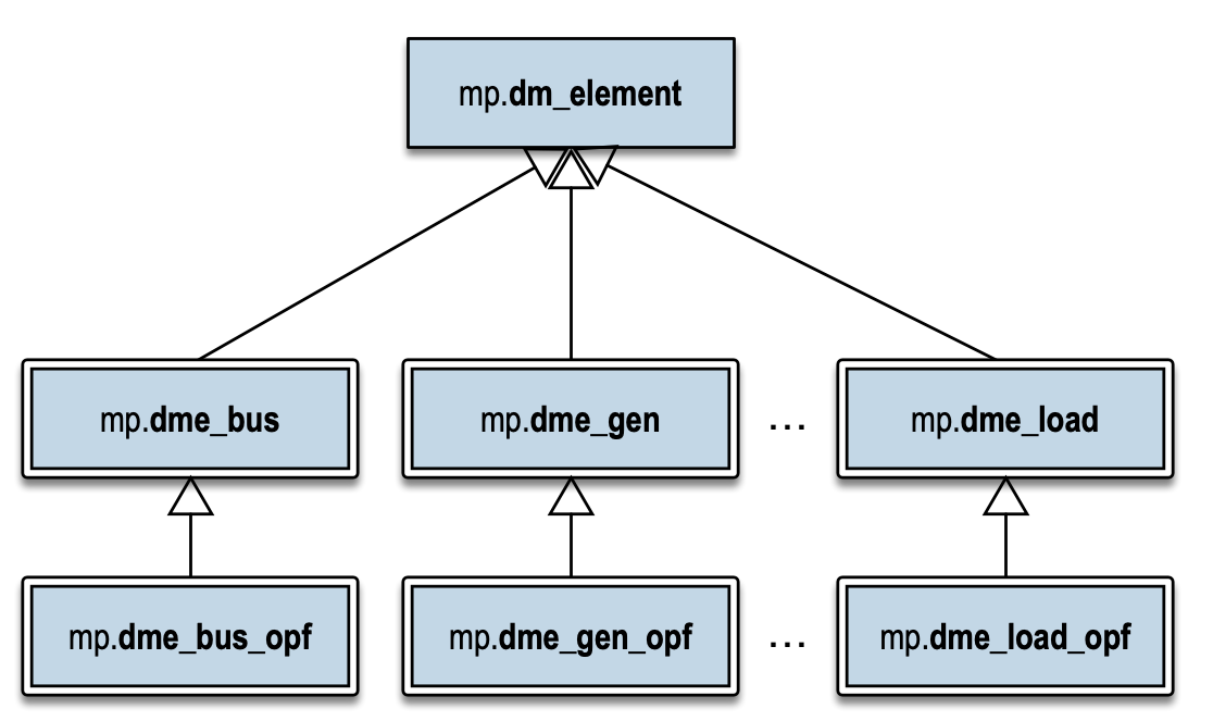
Figure 5.2 Data Model Element Classes
5.2.1. Data Tables
Typically, a data model element has at least one main table, stored in the tab property. Each row in the table corresponds to an individual element and the columns are the parameters. In general, MATPOWER attempts to follow the parameter naming conventions outlined in The Common Electric Power Transmission System Model (CTM) [CTM]. The following parameters (table columns) are shared by all data model elements.
uid – positive integer serving as a unique identifier for the element
name – optional string identifier for the element
status – 0 or 1, on/off-line status of the element
source_uid – implementation specific (e.g. sometimes used to map back to a specific record in the source data)
5.2.2. Properties
The table below includes additional properties, besides the main table tab, found in all data model elements.
Property |
Description |
|---|---|
number of rows in the table, i.e. the total number of elements of the type |
|
number of online elements of the type |
|
vector of row indices of online elements |
|
vector of row indices of offline elements |
|
\(M \times 1\) vector mapping IDs to row indices, where \(M\) is the largest ID value |
|
\(n_r \times 1\) vector mapping row indices to the corresponding index into the |
|
main data table |
5.2.3. Methods
A data model element also has a name() method that returns the name of the element type under which it is entered in the data model (container) object. For example, the name returned for the mp.dme_gen class is 'gen', which means the corresponding data model element object is found in dm.elements.gen.
There are also methods named label() and labels() which return user visible names for singular and plural instances of the element used when pretty-printing. For mp.dme_gen, for example, these return 'Generator' and 'Generators', respectively.
Note
Given that these name and label methods simply return a character array, it might seem logical to implement them as Constant properties instead of methods, but this would prevent the value from being overridden by a subclass, in effect precluding the option to create a new element type that inherits from an existing one.
The main_table_var_names() method returns a cell array of variable names defining the columns of the main data table. These are used by the corresponding data model converter element to import the data.
There are also methods that correspond to the build steps for the data model container object, count(), initialize(), init_status(), update_status(), and build_params(), as well as those for pretty printing output, pretty_print(), etc.
5.2.4. Connections
As described in the Network Model Object section, the network model consists of elements with nodes, and elements with ports that are connected to those nodes. The corresponding data model elements, on the other hand, contain the information defining how these port-node connections are made in the network model, for example, to link generators and loads to single buses, and branches to pairs of buses.
A connection in this context refers to a mapping of a set of ports of an element of type A (e.g. from bus and to bus ports of a branch) to a set of nodes created by elements of type B (e.g. bus). We call the node-creating elements junction elements. A single connection links all type A elements to corresponding type B junction elements. For example, a three-phase branch could define two connections, a from bus connection and a to bus connection, where each connection defines a mapping of 3 ports per branch to the 3 nodes of each corresponding bus.
A data model element class defines its connections by implementing a couple of methods. The cxn_type() method returns the name of the junction element(s) for the connection(s). The cxn_idx_prop() method returns the name(s) of the property(ies) containing the indices of the corresponding junction elements. For example, if cxn_type() for a branch element class returns 'bus' and cxn_idx_prop() returns {'fbus', 'tbus'}, that means it is defining two connections, both to 'bus' elements. The fbus and tbus properties of the branch object are each vectors of indices into the set of 'bus' objects, and will be used automatically to generate the connectivity for the network model.
It is also possible to define a connection where the junction element type is instance-specific. For example, if you had two types of buses, and a load element that could connect to either type, then each load would have to indicate both which type of bus and which bus of that type it is connected to. This is done by having cxn_type() return a cell array of the valid junction element types and cxn_type_prop() return the name(s) of the property(ies) containing vector(s) of indices into the junction element type cell array.