8. Mathematical Model Object
The mathematical model, or math model, formulates and defines the mathematical problem to be solved. That is, it determines the variables, constraints, and objective that define the problem. This takes on different forms depending on the task and the formulation.
- Power Flow
The power flow problem involves solving a system of nonlinear equations for the vector \(\x\).
(8.1)\[\rvec{f}(\x) = \rvec{0}\]For the DC version, the function \(\rvec{f}(\x)\) is linear, so the problem takes the more specific form,
(8.2)\[\param{\rmat{A}} \x - \param{\rvec{b}} = \rvec{0}.\]- Continuation Power Flow
The continuation power flow problem involves tracing the solution curve for a parameterized system of equations, as the parameter \(\lambda\) is varied.
(8.3)\[\rvec{f}(\x, \lambda) = \rvec{0},\]- Optimal Power Flow
The optimal power flow problem, on the other hand, is a constrained optimization problem of the form,
(8.4)\[\begin{split}\min_\x \rvec{f}(\x) \\ \textrm{such that} \qquad \rvec{g}(\x) &= \rvec{0} \\ \rvec{h}(\x) &\le \rvec{0} \\ \param{\x}_{\min} \le \x &\le \param{\x}_{\max}.\end{split}\]This reduces to a simple quadratic program (QP) for the DC OPF case,
(8.5)\[\begin{split}\min_\x \trans{\x} \param{\rmat{Q}} \x &+ \trans{\param{\rvec{c}}} \x + \param{k} \\ \textrm{such that} \qquad \param{\rvec{l}} &\le \param{\rmat{A}} \x \le \param{\rvec{u}} \\ \param{\x}_{\min} & \le \x \le \param{\x}_{\max}.\end{split}\]
8.1. Mathematical Models
A math model object is a container for math model element objects and it is also an MP-Opt-Model object. All math model classes inherit from mp.math_model and therefore also from mp.element_container, opt_model, and mp_idx_manager. Concrete math model classes are task and formulation specific as illustrated in Figure 8.1, and sometimes inherit from abstract mix-in classes that are shared across tasks or formulations. These shared classes are described further in Section 8.3.
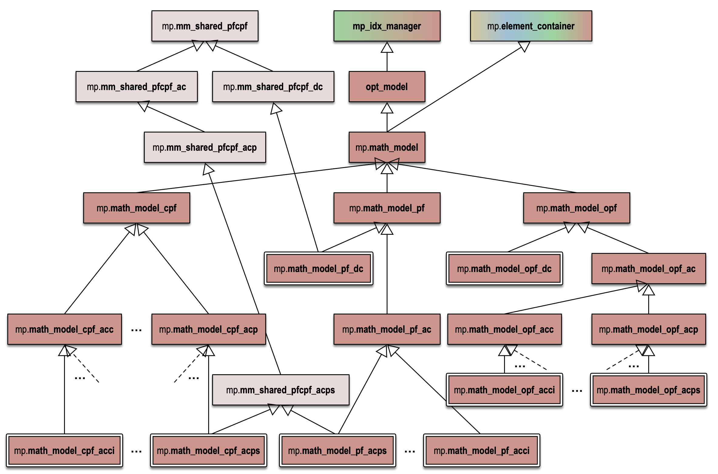
Figure 8.1 Math Model Classes
By convention, math model variables are named mm and math model class names begin with mp.math_model.
8.1.1. Building a Mathematical Model
A math model object is created in two steps. The first is to call the constructor of the desired math model class, without arguments. This initializes the element_classes property with a list of math model element classes. This list can be modified before the second step, which is to call the build() method, passing in the network and data model objects and a MATPOWER options struct.
mm = mp.math_model_opf_acps();
mm.build(nm, dm, mpopt);
The build() method proceeds through the following stages sequentially, looping through each element for the last 3 stages.
Create – Instantiate each element object.
Count and add - For each element object, determine the number of online elements from the corresponding data model element and, if nonzero, add the object to the
elementsproperty of themm.Add auxiliary data – Add auxiliary data, e.g. network node types, for use by the model.
Add variables – Add variables and allow each element to add their own variables to the model.
Add constraints – Add constraints and allow each element to add their own constraints to the model.
Add costs – Add costs and allow each element to add their own costs to the model.
The adding of variables, constraints and costs to the model is done by the math model and model model element objects using the interfaces provided by MP-Opt-Model.
8.1.2. Solving a Math Model
Once the math model build is complete and it contains the full set of variables, constraints and costs for the model, the solver options are initialized by calling the solve_opts() method and then passed to the solve() method.
opt = mm.solve_opts(nm, dm, mpopt);
mm.solve(opt);
The solve() method, also inherited from MP-Opt-Model, invokes the appropriate solver based on the characteristics of the model and the options provided.
8.1.3. Updating Network and Data Models
The solved math model can then be used to update the solved state of the network and data models by calling the network_model_x_soln() and data_model_update() methods, respectively.
nm = mm.network_model_x_soln(nm);
dm = mm.data_model_update(nm, dm, mpopt);
The math model’s data_model_update() method cycles through the math model element objects, calling the data_model_update() for each element.
8.2. Mathematical Model Elements
A math model element object typically does not contain any data, but only the methods that are used to build the math model and update the corresponding data model element once the math model has been solved.
All math model element classes inherit from mp.mm_element. Each element type typically implements its own subclasses, which are further subclassed where necessary per task and formulation, as with the container class.
By convention, math model element variables are named mme and math model element class names begin with mp.mme. Figure 8.2 shows the inheritance relationships between a few example math model element classes. Here the mp.nme_bus_pf_acp and mp.nme_bus_opf_acp classes are used for PF and OPF problems, respectively, with an AC polar formulation. AC cartesian and DC formulations use their own respective task-specific subclasses. And each element type, has a similar set of task and formulation-specific subclasses, such as those for mp.mme_gen.

Figure 8.2 Math Model Element Classes
8.2.1. Adding Variables, Constraints, and Costs
Both the mm container object and the mme element objects can add their own variables, costs and constraints to the model.
For a standard optimal power flow, for example, the optimization variables are added by the container object, since they are determined directly from state variables of the (container) network model object. Similarly, the nodal power or current balance constraints are added by the container since they are built directly from the port injection functions of the aggregate network model.
However, generator cost functions and any variables and constraints associated with piecewise linear generator costs are added by the appropriate subclass of mp.mme_gen, since they relate only to generator model parameters. Similarly, branch flow and branch angle difference constraints are added by the appropriate subclass of mp.mme_branch, since they are specific to branches and are completely independent of other element types.
8.2.2. Updating Data Model Elements
The data in the data model is stored primarily in its individual element objects, so it makes sense that the individual math model element objects would be responsible for extracting the math model solution data relevant to a given element and updating the corresponding data model element. This updating is performed by the data_model_update() method.
The updating of each data model element is done in two steps. First data_model_update() calls data_model_update_off() to handle any offline units (e.g. to zero out any solution values), then data_model_update_on() to handle the online units.
For example, updating the branch power flows and shadow prices on the flow and angle difference limits in the branch data model element is done by data_model_update_on() in the appropriate subclass of mp.mme_branch.